Self-learning Monte Carlo method with Plaquette Ising model

This work is based on https://journals.aps.org/prb/abstract/10.1103/PhysRevB.95.041101.

Self-learning update method

The local update-Monte Carlo method is the most general one, that can be performed on any model, but very slow and inefficient. On the contrary, the global update is the most preferred one due to its speed and efficiency, but can only be applied on specific models. In this paper, the author developed some global update method using self-learning by linear regression. The brief outline follows:

1. Perform original local update using Metropolis-Hastings algorithm to make training data.
   • The data contains the energy of spin configuration, nearest-neighbor correlation, next-nearest-neighbor correlation, and third-nearest-neighbor correlation. I’ll also vary the number of data for training. ($2^{10}, 2^{11}, 2^{12}$)
2. Learn effective Hamiltonian from this data: Using linear regression on energy and spin-correlations.
   • effective Hamiltonian \(\mathcal{H}_{eff} = E_0 - \sum_{k=1}^n \left( J_k\sum_{\langle i,j\rangle_k}s_is_j \right)\): I’ll only consider case $n=1$ and $n=3$.
   • Linear regression: Using python numpy library, $E_0$ and ${J_i}$ is calculated from given training data.

     Jlist, err, _, _ = np.linalg.lstsq(target_mat, E_0, rcond=None)
     

3. Propose a move according to effective Hamiltonian, i.e. create a cluster using $\mathcal{H}_{eff}$.
   • Two different cluster-formation is elaborated below. (section 2.1 & 2.2)
4. Determine whether the proposed moves(=cluster) will be accepted(=flipped), using original Hamiltonian. The acceptance ratio is given by \(\begin{aligned} A_s(a\to b) &= \min\left(1, \frac{p(b)q(a|b)}{p(a)q(b|a)}\right) = \min\left(1, \frac{p(b)p_{eff}(a)}{p(a)p_{eff}(b)}\right) \\&= \min(1, \exp(-\beta\{(E_b-E_b^{eff})-(E_a-E_a^{eff})\})) \end{aligned}\)

However, it is not over yet. We must obtain training data from a critical point, where the local update perform poorly.

• Perform step 1 to get initial training data at temperature higher than critical point, s.t. $T_i=T_c+2$, and perform step 2.
• By obtained effective Hamiltonian, create next training data by doing step 3 and 4 at $T<T_i$. Perform step 2 again.
• Repeat ‘step b’ until the temperature reaches point $T_c$.

Lastly, by derived effective Hamiltonian, we will compare this with the original Hamiltonian, for diverse temperature range. To form a cluster considering only nearest-neighbor($J_1$) is simple, which is just a Wolff cluster method. However, to consider higher order correlation such as next-nearest-neighbors($J_2$) and third-nearest-neighbors($J_3$) is a complex problem. I’ve considered two methods to solve this problem.

Method 1

The first method is to consider nth-NN during formation of cluster, which is by including $J_2$ and $J_3$ correlation directly during the construction of the cluster. The brief scheme of this algorithm is to search the $J_2, J_3$ correlation inside the cluster. This method goes similar to Wolff cluster, however, in the interval, it calculates higher order correlation.

1. Choose a random site $i$. Select the nearest neighbor of $i$, call it $j$.
2. Search for 2nd-NN and 3rd-NN for $j$ , inside the cluster. The number of 2nd-NN and 3rd-NN inside the cluster is each denoted by $n_2, n_3$. The probability to bond site $j$ is $p = 1 - \exp(-2\beta (J_1+n_2J_2+n_3J_3))$.
3. Repeat step 1 for site $j$, if it was in cluster. Keep until no more bond is created.
4. This cluster will be flipped by considering the acceptance ratio of $A_s$ above.

The key point of this cluster formation is the consideration of 2nd-NN and 3rd-NN inside bond-probability.

// Front line same as Wolff cluster...
vector<int> search(size_*size_, 0);
stack[0] = i; search[i] = 1;
while (1) {
	for (int k = 0; k < 4; k++){ 
		p = na[i][k]; 
		n2 = search[na[p][4]] + search[na[p][5]] + search[na[p][6]] + search[na[p][7]]; //J2
		n3 = search[na[p][8]] + search[na[p][9]] + search[na[p][10]] + search[na[p][11]]; //J3
		prob = padd_[5*n2+n3]; // Define probability before, and reference it.
		if (prob>0){
			if (v_[point] == oldspin && dis(gen) < prob) { 
				sh++; 
				stack.at(sh) = point; 
                search[point] = 1; 
                // 'search' array has value 1 at the location of cluster.
				v[point] = newspin; 
		}
	}
}
/* ... : Accept this flip by considering Self-Learning acceptance operator. */
//Finished.

Method 2

The second method is to change the acceptance ratio of cluster flipping; form a cluster regarding $J_1$ correlation, and accept/reject this cluster flip by considering $J_2, J_3$ correlation. This method was inspired by the shift of acceptance ratio during self-learning.

1. Construct Wolff-cluster using only information about 1st-NN, as normal. This step is identical to Wolff-cluster formation.
2. Accept this cluster flip regarding given Hamiltonian, which includes 2nd-NN and 3rd-NN. \(\begin{aligned} A^*(a\to b) &= \min\left(1, \frac{p(b)q(a|b)}{p(a)q(b|a)}\right) = \min\left(1, \frac{p(b)p_{J_1}(a)}{p(a)p_{J_1}(b)}\right) \\&= \min(1, \exp(-\beta[(E_b-E_b^{J_1})-(E_a-E_a^{J_1})])) \end{aligned}\) Where $E^{J_1}$ implies the effective energy calculated using only 1st-NN. This step is similar to self-learning acceptance operator.
3. This cluster flip will again be accepted or rejected regarding $A_s$ above.

For the overall acceptance ratio of cluster, \(A(a\to b) = \min\left(1, \frac{p(b)p_{eff}(a)}{p(a)p_{eff}(b)}\min\left(1, \frac{p_{eff}(b)p_{J_1}(a)}{p_{eff}(a)p_{J_1}(b)}\right)\right)\) where $p$ stands for original Hamiltonian that we are interested in, $p_{eff}$ for effective Hamiltonian, and $p_{J_1}$ for effective Hamiltonian of 1st-NN.

vector<double> v = array; // array: given spin configuration
/* ... : Cluster formation on v */
double ediff1, ediff2; // Two level operator
ediff1 = ((eff_E(v, J, nth) - eff_E(v, J, 1)) 
          - (eff_E(array, J, nth) - eff_E(array, J, 1))) / T; 
// If cluster flip accepted by effective Hamiltonian, go to next step!
if (ediff1 <= 0 || (dis(gen) < exp(-ediff1)) { 
	ediff2 = (((original_E(v, K) - eff_E(v, J, nth)) 
               - (original_E(array, K) - eff_E(array, J, nth))) / T;
    // If cluster flip is accepted by original Hamiltonian, flip!
	if (ediff2 <= 0 || (dis(gen) < exp(-ediff2)) { array = v; } 
	}
//Finished.

To test whether these two methods are acceptable, I performed cluster-formation and compared it to Metropolis algorithm, using below Hamiltonian. (This is because Metropolis algorithm can be applied to any model.) \(\mathcal{H} = -\sum_{k=1}^2\sum_{\langle i,j\rangle_k}J_k s_is_j, \,\text{where } J_1 = 1, \, -0.15<J_2<0.15\)

Below figure shows the comparison of metropolis update and cluster update using method 1 and 2.

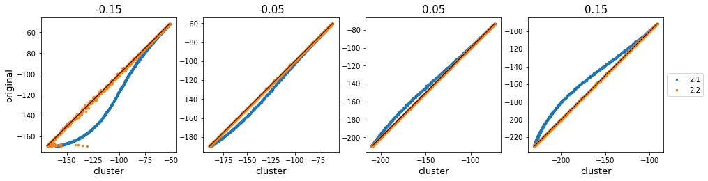
R square	-0.15	-0.05	0.05	0.15
method 1	0.84273832	0.99276231	0.99497835	0.95549145
method 2	0.99684442	0.99996033	0.99996566	0.99994447

As $J_2$ deviates from $0$, method 2.1 diverges from the original value. This implies the detailed balance of this system has not been satisfied. The above table shows the R$^2$-value. In this next-nearest-model, it is clear that the method of changing the acceptance ratio works better. However, I’ll perform both methods on self-learning, and then compare these two.

Result

I’ll mainly perform self-learning on plaquette-Ising model, which is \(\mathcal{H} = -J\sum_{\langle i, j\rangle}s_is_j-K\sum_{ijkl\in\Box}s_is_js_ks_l\) I’ll focus on the case where $K/J = 0.2$. (Both positive and ferromagnetic.)

By performing Metropolis-Hastings algorithm on a plaquette-Ising model of system size 10, 20, and 40, we assume that $T_c = 2.503\pm0.006$, however, I’m going to use $T_c=2.493$ as introduced in this paper.

First, I have performed Metropolis algorithm for fitting plaquette Hamiltonian (I’ll call this original Hamiltonian) into effective Hamiltonian $\mathcal{H} = -\sum_{k=1}^{nth}\sum_{\langle i,j\rangle_k}J_k s_is_j$, differing the size of training data $2^{10}$~$2^{12}$.

R square	$2^{10}$	$2^{11}$	$2^{12}$
$J_1$	0.9977622159345134	0.9979367589474513	0.9980402045898196
$J_1$~$J_3$	0.997696360155469	0.9979543930109472	0.998002372508706

Obviously, using larger training data size ensures high accuracy of the effective Hamiltonian. Indeed, considering 3rd-order correlation during fitting (i.e. fitting to $J_3$) does not seem to have big difference with the $J_1$ consideration. Considering only $J_1$ in this case will work well.

Comparison: method

Method 1

R square	$2^{10}$	$2^{11}$	$2^{12}$
1st-NN	0.9996268876183921	0.9997928031923388	0.9998775706675226
3rd-NN	0.966586965517033	0.9691316899978449	0.9712051149363949

$H_{eff}$	J1	J2	J3
1st-NN	1.112$\pm$0.001	.	.
3rd-NN	1.221$\pm$0.003	-0.0682$\pm$0.004	-0.017$\pm$0.004

Considering 2nd and 3rd order spin correlation while forming a cluster does not seem to ensure an accurate result. It shows some deviation from the original-metropolis method. This cluster formation method in inappropriate in this case.

Method 2

R square	$2^{10}$	$2^{11}$	$2^{12}$
1st-NN	0.9996497667105083	0.9997915851810159	0.9998742868415753
3rd-NN	0.9980529594579894	0.9994300500264944	0.9996079715633984

$H_{eff}$	J1	J2	J3
1st-NN	1.1126$\pm$0.0006	.	.
3rd-NN	1.26$\pm$0.01	-0.099$\pm$0.009	-0.009$\pm$0.003

The second method of forming a cluster are more accurate, and works well during fitting $J_3$. Overall, implementing method 2.2 into self-learning performs much better, so I’m going to choose this method for the following analysis.

Analysis

To understand the self-learning exactly, we must know its overall situation. First, I’ll obtain the actual acceptance rate of this model, to compare two cases of effective Hamiltonian. Then, I’ll calculate the integrated autocorrelation time for each case, and compare it with the original Metropolis method.

Acceptance ratio

Knowing the acceptance rate of a model is important, since rejection-dominant model will not work efficiently. \(A(a\to b) = \min\left(1, \frac{p(b)p_{eff}(a)}{p(a)p_{eff}(b)}\min\left(1, \frac{p_{eff}(b)p_{J_1}(a)}{p_{eff}(a)p_{J_1}(b)}\right)\right)\) To compare the overall acceptance rate, I performed cluster formation by different sizes and different steps at the critical temperature. A cluster was created based on the obtained values from self-learning linear regression.

Below, I had compared the acceptance rate for two types of effective Hamiltonian, in various system size. (Consideration of only $J_1$ versus consideration up to $J_3$.) The leftmost plot shows the acceptance ratio of level 1, which is the ‘$J_1$-cluster flip based on effective Hamiltonian’. The center plot shows the acceptance ratio of level 2, which is the ‘effective-cluster flip based on the original Hamiltonian’. The rightmost plot shows the overall acceptance ratio.

Level-1 acceptance ratio is related to the similarity of the energy level of $J_1$ cluster and the effective Hamiltonian. (Actual flip happens here.) Level-2 acceptance ratio is related to ‘how much the fitting was successful.’ The closer the effective Hamiltonian with original Hamiltonian, the more it will become accepted. The overall acceptance ratio explains how successful was our cluster formation is.

Below figure shows the same result, however, x-axis has logarithmic scale.

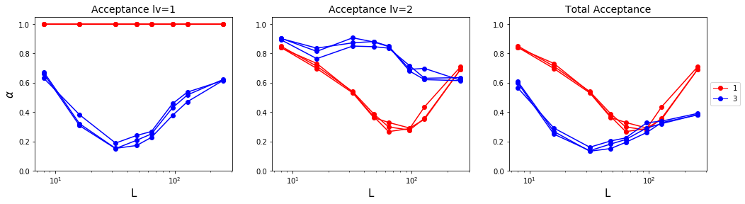
Surprisingly, level-1 acceptance ratio dropped and elevated steadily for $J_3$ case. Moreover, for level-2 acceptance ratio, $J_1$ case also showed some unexpected increase. (There was no surprise on level-2 acceptance ratio of $J_3$ case.) Overall, both cases showed some unique patterns of acceptance ratio.

We could carefully suggest that this is related to the cluster’s size. For small-sized systems, cluster size is also quite small, which makes it more likely to be accepted by original Hamiltonian. For a slightly larger system, it doesn’t work well since the cluster size also gets big enough to be rejected. However, as the system gets large enough, the cluster size doesn’t seem to affect this acceptance rate. We might guess that cluster size is bounded anyway.

Another analysis is solely about level-2 acceptance rate. Clearly, at a smaller size, $J_3$-effective Hamiltonian is more likely to be accepted than the $J_1$-effective Hamiltonian. We could simply claim that $J_3$ fitting is more accurate than $J_1$ fitting when the system size is small. However, as the system gets larger, there was a reverse; $J_1$ effective Hamiltonian seems to work well. The total acceptance rate shows that $J_1$ fitting will work well during self-learning.

Overall, there seem to have some bounded limit for acceptance rate.

Autocorrelation time

The paper demonstrates that the self-learning method is useful due to its efficiency and reduction in autocorrelation time. To check this fact, I calculated integrated autocorrelation time for various sizes; 8, 12, 16, 24, 32. There are two cases to compare: one is $J_1$-effective Hamiltonian, and the other is $J_3$-effective Hamiltonian. I would compare this result with the original Hamiltonian, which was performed using Metropolis algorithm. The calculation was held at the critical point.

For $J_1$-fitting, the exponent $z = 1.07878$. For $J_3$-fitting, the exponent $z = 2.96047$. Compare to original metropolis exponent $z = 1.87278$, $J_3$ fitting has more autocorrelation. We can assume that due to its low acceptance rate, cluster formation was not fully reflected, which leads to huge autocorrelation time. However, the $J_1$-fitting showed great reduction on autocorrelation time. We can conclude that self-learning simulation on plaquette-Ising model is successful.

It was surprising that original metropolis exponent didn’t reach value $2$. I have only conducted this calculation on small-size systems ($L\leq 32$). This leads to major error in estimation of exponents.

Reference

• J. Liu, Y. Qi, Z. Y. Meng, and L. Fu, Self-learning Monte Carlo method, Phys. Rev. B, vol. 95, no. 4 (2017)