Classical Ising model with MCMC

Classical Ising model

Classical Ising model is briefly explained in https://aadeliee22.github.io/physics/tsp-presentation/#classical-ising-model. This model is the simplest model of a magnet. Here, I will invest some special thermal properties of this model, with second-order phase transition and critical point.

Background

Some thermodynamic and statistical backgrounds, as well as Monte Carlo methods.

First, by determining Helmholtz free energy of system $\mathcal{F} = -kT\ln Z$, we know that \(S = -\left(\frac{\partial \mathcal{F}}{\partial T}\right)_{V, N}, P = -\left(\frac{\partial \mathcal{F}}{\partial V}\right)_{T, N}, \mu = -\left(\frac{\partial \mathcal{F}}{\partial N}\right)_{T, V}\) Moreover, using these, we now obtain other quantities that may use as order parameters. \(U = -\frac{1}{Z}\frac{\partial Z}{\partial\beta} = -\frac{\partial}{\partial\beta}\ln Z = -T^2 \frac{\partial (\mathcal{F}/T)}{\partial T} = \langle E \rangle \\ \begin{aligned} C &= T \frac{\partial S}{\partial T} = -\beta \frac{\partial S}{\partial \beta}= \frac{\partial U}{\partial T} = k\beta^2 \frac{\partial^2}{\partial \beta^2}\ln Z \\&=k\beta^2\left(\frac{1}{Z}\frac{\partial^2}{\partial\beta^2}Z - \left[ \frac{1}{Z}\frac{\partial}{\partial \beta}Z\right]^2\right) =k\beta^2(\langle E^2\rangle - \langle E\rangle^2) \end{aligned} \\M = \frac{\partial \mathcal{F}}{\partial B} = \left\langle \sum_i s_i \right\rangle, \;\; \chi = \frac{\partial\langle M\rangle}{\partial B} = \beta (\langle M^2\rangle - \langle M \rangle ^2)\) where $U$ is internal energy, $C$ is specific heat capacity, and $M$ is magnetization, $\chi$ is magnetic susceptibility. Therefore, by knowing partition function, we could drive almost all quantities that we need.

Mean field approximation of $d$-dimensional lattice is explained in https://aadeliee22.github.io/physics/tsp-presentation/#mean-field-theory-for-d-dimensional-lattice. Here, I will show exact solution for 1D lattice.

Consider 1-dimensional Ising model of periodic boundary that has $N$ sites. Given Hamiltonian, the partition function is \(\begin{aligned} Z =& \sum_{\{\vec{s}\}}\exp(\beta J (s_1s_2 + \cdots + s_N s_1)+ \beta B(s_1+\cdots+s_N)) \\=& \sum_{\{\vec{s}\}}\exp(\beta J (s_1s_2 + \cdots + s_N s_1)+ \frac{1}{2}\beta B((s_1+s_2)+\cdots+(s_N+s_1)) \\=& \sum_{\{\vec{s}\}}\underbrace{\exp(\beta Js_1s_2+\frac{1}{2}\beta B(s_1+s_2))}_{\langle s_1|T|s_2\rangle}\cdots\underbrace{\exp(\beta Js_Ns_1+\frac{1}{2}\beta B(s_N+s_1))}_{\langle s_N|T|s_1\rangle} \\=& \sum_{s_1}\cdots\sum_{s_N}\langle s_1|T|s_2\rangle\cdots\langle s_N|T|s_1\rangle = \sum_{s_1}\langle s_1|T|s_1\rangle = \text{Tr}(T^N) = \sum\lambda_i^N \end{aligned}\)

The $T$ part acts like a matrix, as each spin is either $1$ or $-1$. \(T = \begin{array}{c|cc}s_i, s_{i+1}&+1 & -1 \\\hline +1 & e^{\beta(J+B)} & e^{-\beta J} \\-1 & e^{-\beta J} & e^{\beta(J-B)} \end{array}\) This matrix has eigenvalue of \(\lambda = e^{\beta J}\cosh \beta B\,\pm\sqrt{e^{2\beta J}\cosh^2\beta B-2\sinh2\beta J}\) For $B=0$, $\lambda = e^{\beta J}\pm e^{-\beta J}$. Using this, we can calculate free energy and internal energy each. \(\mathcal{F} = -kT\ln Z = -\beta N\ln 2\cosh\beta J \\ U = -\frac{\partial}{\partial \beta}\ln Z = -JN\tanh\beta J\)

Markov Chain Monte Carlo

Exact partition function is difficult to figure out, however, by statistical Monte Carlo simulations, it is able to solve it. Generally, we use a Markov chain. It requires careful design, as it must satisfy some properties.

The first-order Markov chain only depends on the last previous state(conditional probability) and can be described by transition function. \(p(x^{(k+1)}|x^{(1)}, \cdots,x^{(k)}) \equiv p(x^{(k+1)}|x^{(k)})\equiv T_k(x^{(k)}, x^{(k+1)}), \;\text{where }k\in 1, \cdots,M\) This chain is homogeneous if $\forall i, j, \,T_i = T_j$.

A distribution is invariant/stationary when a transition function of the chain leaves the distribution unchanged, i.e. \(p'(x) = \sum_{x'}T(x', x)p'(x')\) Designing a transition operator that makes distribution stationary is important in our case. The transition operator satisfies detailed balance by \(p'(x)T(x, x') = p'(x')T(x', x)\) If this detailed balance is satisfied, the distribution is stationary under $T$. Moreover, if the distribution $p(x^{(k)}|x^{(0)})\to p’(x)$ (invariant) when $k\to\infty$, then the chain has property ergodicity. A poorly designed operator might divide a set into certain states. That is, the distribution can reach any state after a long time from any state.

In general, the transition operator from $a$ to $b$ is given by $T(a\to b) = A(a\to b)q(b|a)$.

Local update

Metropolis-Hastings algorithm is explained below.

We want to obtain $x^{(1)}\mapsto x^{(2)}\mapsto \cdots\mapsto x^{(m)}\cdots$.

• First, initialize, $\tau=1, \, x^{(\tau)}=?$.
• Propose $x’\sim q(x’,x^{(\tau)})$.
• Accept $x’$ with an acceptance ratio $A(x^{(\tau)}\to x’) = \min\left(1, \frac{p(x’)q(x^{(\tau)},x’)}{p(x^{(\tau)})q(x’,x^{(\tau)})}\right)$.
• If accepted, $x^{(\tau+1)} = x’$. Else, $x^{(\tau+1)} = x^{(\tau)}$.
• Repeat the above steps.

In our local update, a proposal is given by $q(b|a) = \text{constant}$. I’ll briefly explain the scheme of this algorithm.

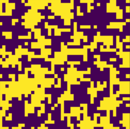
1. Define lattice size ($L$) and nearest-neighboring index. Initialize each spin site randomly or like chess-board; which has maximum energy level. (This will prevent super-cooling.) The nearest-neighboring index array will contain information of periodic boundary condition.
2. Define Monte-Carlo-one-step(1 MC-step) as following:
   • pick one spin site (randomly or checkerboard-style) and flip it.
   • Calculate the energy difference ($=\Delta \mathcal{H}$).
   • If energy difference less than 0, accept the spin-flip. Else, accept it by the probability of $\exp(\Delta\mathcal{H}/kT)$.
   • Perform the above steps for the whole spin site; which will be $L^2$.
3. Calculate important thermodynamic quantities:
   • Before calculation, perform 2000~2500 MC-steps to obtain an accurate value.
   • Calculate magnetization and energy for 10000 times. For each data, throw a few steps according to the autocorrelation time. (e.g. Metropolis: $\theta \sim L^2$, Cluster: $\theta \sim L^{0.44}$) Without this throwing process, we will experience a certain bias of the observed value.
   • Calculate magnetization, magnetic susceptibility, energy, specific heat…etc.
4. Do the above steps for each temperature. Invest some quantities near the critical point.

Global update: Cluster

Well-known local updates such as Metropolis update takes tremendous time and large autocorrelation between each state. We’ll propose the most successful global update method, which is a cluster update. There are some fundamentals(Fortuin-Kasteleyn cluster decomposition) to discuss before explaining the algorithm.

First, let $H = -\sum_{\langle i, j\rangle}s_is_j$ and $Z = \sum_{{s}}e^{-\beta H}$. Remove interaction between fixed nearest-neighboring site of $\langle l, m\rangle$ : $H_{l,m} = -\sum_{\langle i, j\rangle\neq \langle l, m\rangle} s_is_j$. Define new partition function, considering rather $s_i, s_j$ are same or different. \(Z_{l, m}^{=}=\sum_{\{s\}}\delta_{s_l, s_m}e^{-\beta H_{l,m}}, \; Z_{l, m}^{\neq}=\sum_{\{s\}}(1-\delta_{s_l, s_m})e^{-\beta H_{l,m}}\)

The original partition function is $Z = e^\beta Z_{l, m}^=+e^{-\beta}Z_{l, m}^\neq$.

Moreover, define $Z_{l,m}^{ind} = \sum e^{-\beta H_{l,m}} = Z_{l,m}^= + Z_{l,m}^\neq$, then partition function $Z = (e^\beta-e^{-\beta})Z_{l,m}^=+e^{-\beta}Z_{l,m}^{ind}$

Since $Z^=$ contains only when $s_l=s_m$, and $Z^{ind}$ contains no restriction for spin-links, the weighing factors can be considered as probabilities of bond between site $l, m$. \(p_{bond} = 1-e^{-2\beta}, \;Z = \sum p^b(1-p)^n 2^N\)

By using the above probability, one can create a cluster for a simple Ising model. I’ll introduce Wolff-cluster update, which has proposal $q(b|a)/q(a|b) \equiv p(b)/p(a)$. (And has acceptance ratio $=1$.)

1. Choose a random site $i$, and select nearest-neighbor $j$.
2. If $s_i =s_j$, bond to cluster with probability $p = 1-e^{-2\beta J}$.
3. Repeat step 1 for site $j$, if it was in the cluster. Keep until no more bond is created.
4. Flip the entire cluster.

// na = neighbor index array
int i = size*size * dis(gen);
int sp = 0, sh = 0;
double point;
double prob = 1 - exp(-2*J/T);
double oldspin = v[i], newspin = -v[i]; 
vector<int> stack(size*size, 0);
stack[0] = i; search[i] = 1; v[i] = newspin;
while (1) {
	for (int k = 0; k < 4; k++){
		point = na[i][k];
		if (v_[point] == oldspin && dis(gen) < prob) { 
			sh++; 
			stack.at(sh) = point;
			v[point] = newspin; 
		}
	}
}

Ising model Analysis

Finite size scaling

For the finite-size system, the phase transition is smooth and inaccurate, which needs some additional interpretation. For each pseudo-critical temperature at a certain size, we can guess the accurate critical temperature. Usually, a genuine value of critical point can only be obtained from an infinite system.

We can find a singular point of free energy. This can be expressed as a function of size and temperature. \(F(L, T) = L^{(a-2)/\nu}\mathcal{F}((T-T_c)L^{1/\nu})\) Calculation from free energy, we have nice scaling factors. \(M = L^{-\beta/\nu} \tilde{M}((T-T_c)L^{1/\nu}) \\ \chi = L^{\gamma/\nu}\tilde{\chi}((T-T_c)L^{1/\nu}) \\ C = L^{\alpha/\nu}\tilde{C}((T-T_c)L^{1/\nu})\) Ising model’s critical exponents are known as $\alpha = 0,\; \beta = 1/8,\; \gamma = 7/4,\; \nu = 1$. Moreover, $T_c=2/\ln(1+\sqrt{2})\simeq2.2692 $.

Here, I’m scaling using $\chi$. Plot $(T-T_c)L^{1/\nu}$ versus $\chi L^{-\gamma/\nu}$ to draw function $\tilde{\chi}$, and find the maximum point $y_{max}$. At this point, we can figure out real critical temperature by $y_{max} = (T_{L}-T_c)L^{1/\nu}$ ($T_{L}$: pseudo-critical point at size $L$.) Plotting $L^{-1/\nu}$ versus $T_L$ will predict the real critical temperature.

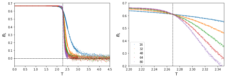
By examining higher order Binder cumulant $B_L$, we can invest $T_c$ more precisely. \(B_L = 1 - \frac{\langle m^4\rangle}{3\langle m^2\rangle^2}\)

As system size goes to infinity, $B_L\to0$ for $T>T_c$ and $B_L\to2/3$ for $T<T_c$. This quantity shows clear convergence near critical point.

Error analysis: Jack knife

As we calculate functions which has a dependency on the previous state(~autocorrelation), normal calculation of error doesn’t work. We have to implement a new error-analyzing method for a given quantity $x$.

1. Calculate average $\langle x\rangle$.
2. Divide data into $k$ blocks (called binning); block size must be bigger than the autocorrelation time, to eliminate the impact of correlation.
3. For each block $i = 1, \cdots, k$, calculate $x^{(i)} = \frac{1}{k-1} \sum_{j\neq i} x_j$
4. Estimate error: $\delta_x^2 = \frac{k-1}{k}\sum_{i=1}^k (x^{(i)}-\langle x\rangle)^2$

As this method slices data into several blocks, its name is Jack knife. In general, the error estimated from Jack knife method is larger than the normal error (standard deviation, usually.) Jack knife error usually $\tau_{int}$ times larger than the calculated error.

Autocorrelation time

The autocorrelation function is the correlation of some parameter $X$ with delayed-itself as a function of time. \(\langle X(0) X(t)\rangle - \langle X\rangle ^2 = C(t) = \frac{1}{N-t}\sum_{n=1}^{N-t}(X_n - \langle X\rangle)(X_{n+t}-\langle X\rangle) \sim e^{-t/\tau_{exp}}\) For error analysis, we usually use integrated autocorrelation time. \(\tau_{int} = \frac{1}{2} + \sum_{t=1}^\infty C(t)\lesssim \tau_{exp} \;(\sim \text{for pure exponential function})\) By fast Fourier transformation (FFT), we can sum up the values in reduced time. Calculating the integrated autocorrelation time of the given parameter takes only $O(\log N)$ time. Algorithm for estimating autocorrelation time refered from ref

Result

The classical Ising model with $J=0$ is used here. First, a comparison between local/global update was conducted. For the next step, an examination of some important quantities of different sizes was done.

Comparison: update method

A local update was performed using the Metropolis algorithm, and the global update was by the Wolff cluster algorithm. I have calculated the accuracy of the global update, and the efficiency of the global update compare to the local update.

R-square

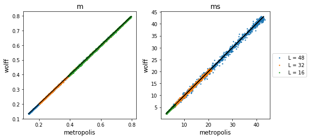
System size 16, 32, 48 was used to compare R square.

Magnetization and Magnetix susceptibility comparison, where big dots are from Metropolis and small dots from cluster method.

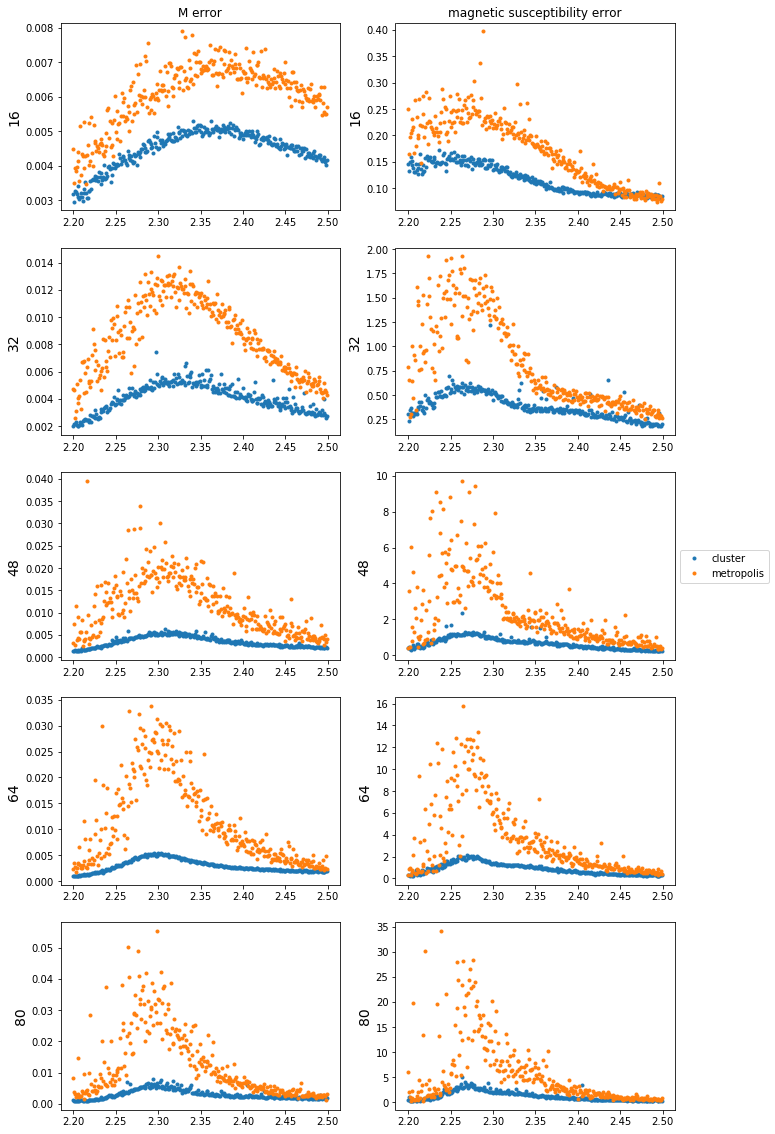
Error comparison

The orange dots are error calculated from the Metropolis, and blue ones are error from the clustering algorithm. There is a clear relation between autocorrelation time and the error obtained by jack knife; metropolis error was much bigger than cluster error, and also, error at the critical point was largest among given temperature range.

Integrated Autocorrelation time

System size of 8, 16, 32, 64, 128 was used here to compare autocorrelation. Parameter such as magnetization and magnetic susceptibility was used to calculate integrated autocorrelation time for each algorithm. The calculation was on a critical point, which has the worst autocorrelation.

Starting with magnetization autocorrelation time,

Autocorrelation	Metropolis	Cluster
function
integrated time

Below graphs shows $\tau_{int}\sim L^z$. (z = 0.44479 for cluster, z = 2.00119 for metropolis.)

Moreover, I calculated the integrated autocorrelation time for magnetic susceptibility. (z = 0.33127 for cluster, z = 2.0587 for metropolis.)

Cluster algorithm works much better than the Metropolis one. Autocorrelation time for Metropolis diverges faster than the clustering algorithm. At system size 128, it gets terribly inefficient. As the clustering algorithm has less autocorrelation time, we can throw fewer steps to obtain results that we need. For these reasons, I’m going to use the Wolff cluster method for investing the Ising model’s finite size effect.

Comparison: lattice size

Thermodynamic quantities

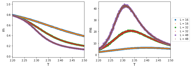
Overall, magnetization was used here to calculate some quantities, such as magnetic susceptibility and Binder cumulant of magnetization. (left) Magnetization by different size (center) Magnetic susceptibility (right) Magnetic susceptibility in log scale.

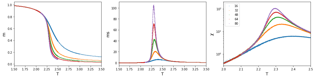
Obviously, as size increases, the more it acts as an infinite size. Magnetization drops exponentially at a critical point. Also does magnetic susceptibility. As the size grows, magnetic susceptibility diverges at a critical point. However, we can figure out some subtle critical-temperature shifts as varying system size. To accurately obtain a critical point, we must perform some other analysis.

$B_L$ with $m$

The vertical dashed line (–) represents the critical temperature, where $T_c = 2/\ln(1+\sqrt(2))\simeq2.2692$. At critical point, Binder value converges.

Finite size scaling with $\chi$

The value of maximum y position(red dashed line): 1.968705

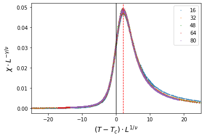
The above result shows that the well-known critical exponents of the Ising model match exactly with our model, which implies our simulation is successful.

To obtain genuine critical temperature, we must do ‘finite size scaling’ from each pseudo-critical values. The plot shows the linear fitting curve. The $y$-intercept of these lines indicates the predicted critical temperature.

• include all points: $2.053837x+2.268260$
• exclude point $L=16$: $2.059052x+2.268162$
• exclude point $L=16, 32$: $1.430204x+2.277027$

By considering some standard deviation and errors, we could conclude that the critical temperature is about $T_c = 2.268 \pm 0.004$. Our result deviates only 0.0012 from well-known value.

Reference

1. M. E. J. Newman and G. T. Barkema, Monte Carlo methods in statistical physics. Oxford: Clarendon Press, 2001.
2. L. E. Reichl, A modern course in statistical physics. Weinheim: Wiley-VCH, 2017.
3. C. J. Adkins, An introduction to thermal physics. Cambridge: Cambridge University Press, 2004.
4. D. P. Landau and K. Binder, A guide to Monte Carlo simulations in statistical physics. Cambridge, United Kingdom: Cambridge University Press, 2015.
5. K. Rummukainen, in Monte Carlo simulation methods, 2019.
6. F. Wood, “Markov Chain Monte Carlo (MCMC),” in C19 MACHINE LEARNING - UNSUPERVISED, Jan-2015.
7. D. Foreman-Mackey, “Autocorrelation time estimation,” Dan Foreman-Mackey [Online]. Available: https://dfm.io/posts/autocorr/. [Accessed: 20-Aug-2020].