Machine learning prediction of metal-insulator transition in DMFT Hubbard model

In this research, we aim to investigate the relationship between the metal-insulator transition andthe discrete bath orbitals calculated in the dynamical mean-field theory with exact diagonalizationby applying machine learning approaches. We train the neural network with raw data without preliminary physical knowledge to find the hidden patterns of the data by itself, and finally to construct the physics from it.

This work is a collaborative work, and my contribution is listed here:

• Conducting DMFT-NRG and obtain data from it.
• Train neural network model with DMFT-NRG hybridization function, calculate accuracy
• Transformation of weight matrix to ensure that the input layer receives the Matsubara frequency domain data.
• Test our neural network model with the hybridization function on the Matsubara frequency domain.
• Analyze the structure of neural network.

From this part, my co-worker contribution part.

• Find the quantity $S_2$, which can be considered as an effective order parameter.
• Discriminate phase using $S_2$ in other lattice geometries, confirm that it is the effective order parameter.

Introduction: DMFT

Dynamic mean-field theory is the method to describe the properties of the strongly correlated materials. DMFT maps many-body lattice problem into many-body local problem which is the impurity problem. Using the Anderson impurity model, it is now solvable with the self-consistency equation. Various solvers are such as NRG(numerical renormalization group), ED(exact diagonalization), or QMC(quantum Monte-Carlo).

Especially, DMFT-ED has advantages of sign-problem-free, enabling direct access to the GReen’s function on real-frequency axis without numerical analytic continuation technoque. DMFT-ED works with a few bath orbitals mapping from the lattice model to the impurity model. We focus on the relationship between the sests of bath parameters and metal-insulator transition.

DMFT-NRG is the method that can calculate the exact spectral function on the real frequency. For the Bethe lattice, the spectral function is equivalent to the imaginary part of the hybridization function, and therefore, we will predict the phase transition of the DMFT on the Hubbard model by training a simple neural network model with the hybridization function. Furthermore, we will test this model on the Matsubara frequency.

DMFT-NRG calculation

Dynamical Mean Field Theory with Anderson impurity model solver as ‘numerical renormalization group’ method. One DMFT loop consists of the following steps.

1. Make DMFT approximation on self energy $\Sigma\simeq\Sigma_{imp}$
2. Calculate local Green function
3. Compute hybridization function, and new impurity Green function.
4. Calculate new $\Sigma$ using self consistency

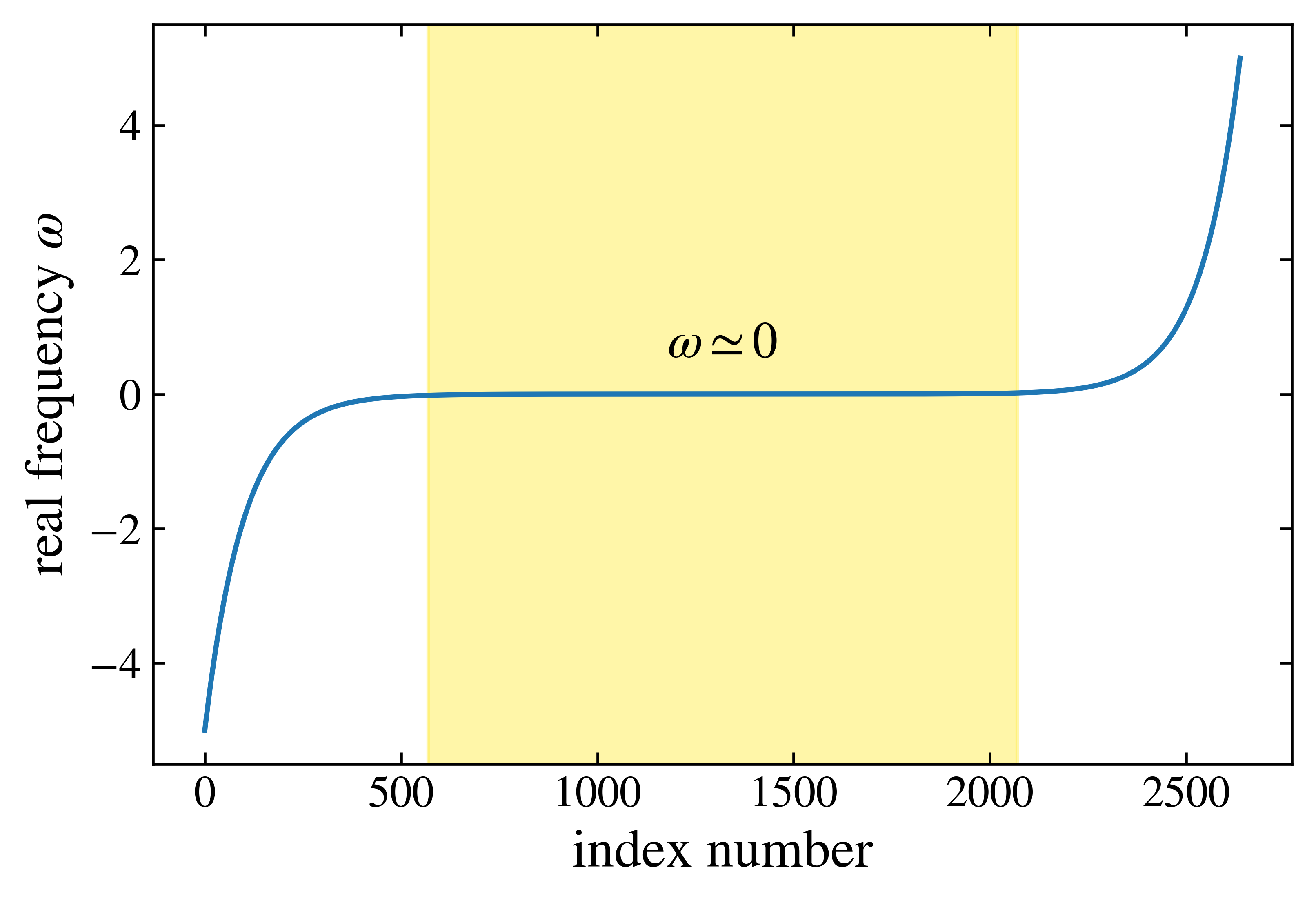
In Bethe lattice, self consistency: $\Gamma = D^2 G/4$. Moreover, DMFT-NRG has characteristics of logarithmic discretization, which is employed during the calculation to ensure its continuity near zero frequency. (Vast majority of the data is centered near zero frequency.)

Implementing broyden method with hybridization function have increased the speed of calculation. \(\Gamma_{out} = dmftstep(\Gamma_{in}))\\ 0 = F(\Gamma_{new}) = dmftstep(\Gamma_{in})-\Gamma_{in}\)

Finally, calculated phase transition points $U_{c1}$ and $U_{c2}$ are

$1/T$	100	1000	10000
$U_{c1}$	2.200	2.225	2.250
$U_{c2}$	2.50	2.69	2.9

Results

Metal-insulator transition and bath parameters

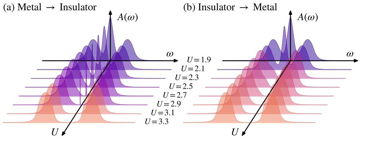
The Hamiltonian of the single orbital Hubbard model is \(H=-t\sum_{i,j,\sigma}{\bigg(c^{\dagger}_{i\sigma}c_{j\sigma}+c^{\dagger}_{j\sigma}c_{i\sigma}\bigg)+U\sum_{i}{n_{i\uparrow}n_{i\downarrow}}}+\mu\sum_{i\sigma}n_{i\sigma}\) where $\mu$ is the chemical potential, $t$ is the hopping element, and $U$ is the on-site interaction. The system experiences Mott transition by tuning $U$ in half-filling ($\mu=U/2$). The above figure displays the evolution of spectral function $A(\omega)$ through $U$ for the Bethe lattice.

From DMFT-ED, the bath parameters is fitted to discribe lattice Green’s function, however, this parameters have many local minimums in the finite bath size. To circumvent these, we introduce neural network that discriminates phase based on hybridization function.

Training neural network

The scheme of training and testing the neural network model is illustrated below. As \(\Gamma(i\omega_n)-\sum_{k=1}^{n_b}\frac{V_{k}^{2}}{i\omega_n-\epsilon_{k}}\) we first employ $\Gamma(i\omega_n)$, the hybridization function on the Matsubara frequency axis as the training set.

However, the test accuracy for transition point $U_{c2}$ is relatively lower than the accuracy for $U_{c1}$. This result implies that the neural network model has failed to learn the pattern of metal-insulator phase transition.

To increase the model accuracy of predicting phase transition, we employ another neural network that predicts the metal-insulator phase transition based on $\Gamma(\omega)$, since the shape of the spectral function directly reflects the phase transition. The input layer of the model receives the imaginary part of the hybridization function, and gives the probability of being in each phase as an output. (The output vector consists of $P_{metal}$ and $P_{insul}$.)

1. Training step: the input layer receives the imaginary part of the hybridization function on the real frequency domain. The model is tested to see the accuracy of prediction, on real frequency domain.
2. Transformation: $\mathbf{W}^{(1)}\to\mathbf{W}^{\prime(1)}$. Details in here.
3. Testing step: the input layer receives the imaginary part of the hybrdization function on the Matsubara frequency domain. We use data obtained from DMFT-NRG(use spectral function to extract Green function on the Matsubara frequency domain) and DMFT-ED for testing model.

\(\mathbf{y}=\mathbf{W}^{(1)}(\Delta(\omega_n+i\eta))^{\mathbf{T}} + \mathbf{b}^{(1)}, \\ \mathbf{z}=\mathbf{W}^{(2)}\sigma(\mathbf{y})+ \mathbf{b}^{(2)}, \\ \mathbf{P}=\sigma(\mathbf{z})\) where $\sigma(x) = 1/(1+\exp(-x))$ is the sigmoid function. The training set consists of the hybridization function from DMFT-NRG, for given on-site interactions $U_I^{(tr)}=\lbrace u\mid 3.0\leq u\leq 5.0\rbrace$ and $U_M^{(tr)}=\lbrace u\mid 0.5\leq u\leq 2.0\rbrace$, which excludes the intermediate region of phase coexistence. Furthermore, we choose three different kinds of models, with various complexity; Neural network with one hidden layer of hidden node $N_h=100$, $N_h=10$, and logistic regression with no hidden layer. This training scheme is illustrated below Fig(a).

After transformation of the weight matrix, we test the model to see whether it works well on the Matsubara frequency domain.

Test data, Bethe	DMFT-NRG	DMFT-ED
$T$	$0.0001$	$0.0001$

Fig(b,c) shows our neural network with one hidden layer works well on the Matsubara frequency domain, as well as on the real frequency domain. Surprisingly, Fig(c) also shows that the logistic regression model works well on the Matsubara frequency domain, having high accuracy of predicting the phase transition points.

Transformation of the weight matrix

This step ensures that the testing-step model receives data on the Matsubara frequency domain. The formula below is based on the Bethe lattice condition. \(\begin{align*} \text{Im}\Delta(i\omega_n) &= \frac{1}{4}\text{Im}G(i\omega_n) = \text{Im}\left(\frac{1}{4}\int_{-\infty}^\infty\frac{A(\omega')d \omega'}{i\omega_n-\omega'}\right) \\&= -\text{Im}\left(\frac{1}{\pi}\int_{-\infty}^\infty\frac{\text{Im}\Delta(\omega')d \omega'}{i\omega_n-\omega'}\right) \\ \mathbf{W}^{(1)}(i\omega_n) &= -\text{Im}\left(\frac{1}{\pi}\int_{-\infty}^\infty\frac{\mathbf{W}^{(1)}(\omega')d \omega'}{i\omega_n-\omega'}\right) \end{align*}\)

Test: on the real frequency domain

After training, we have simply tested whether the model works well on the real frequency domain. Test data from DMFT-NRG. We have used 4 kinds of test data in this section.

As shown below, test outputs are quite awesome!

Test data, DMFT-NRG	Bethe	Cubic
$T$	$0.01, \;0.001, \;0.0001$	$0.0001$

Neural network, $N_h=100$

Neural network, $N_h=10$

Logistic regression

Analyzing the neural network

We claim that there is an universal pattern that can be used in recognizing phase transition. Below figure illustrates (left) the heat maps for the weight matrix $\mathbf{W}^{(1)}(\omega_n)$, (right) and its kernel density estimation of $j$-th node(row) of the weight matrix $\mathbf{W}^{(1)}(\omega)$. Each row indicates different models; Neural network with one hidden layer, hidden node number of (a) $N_h = 100$, (b) $N_h=10$. (c) Logistic regression.

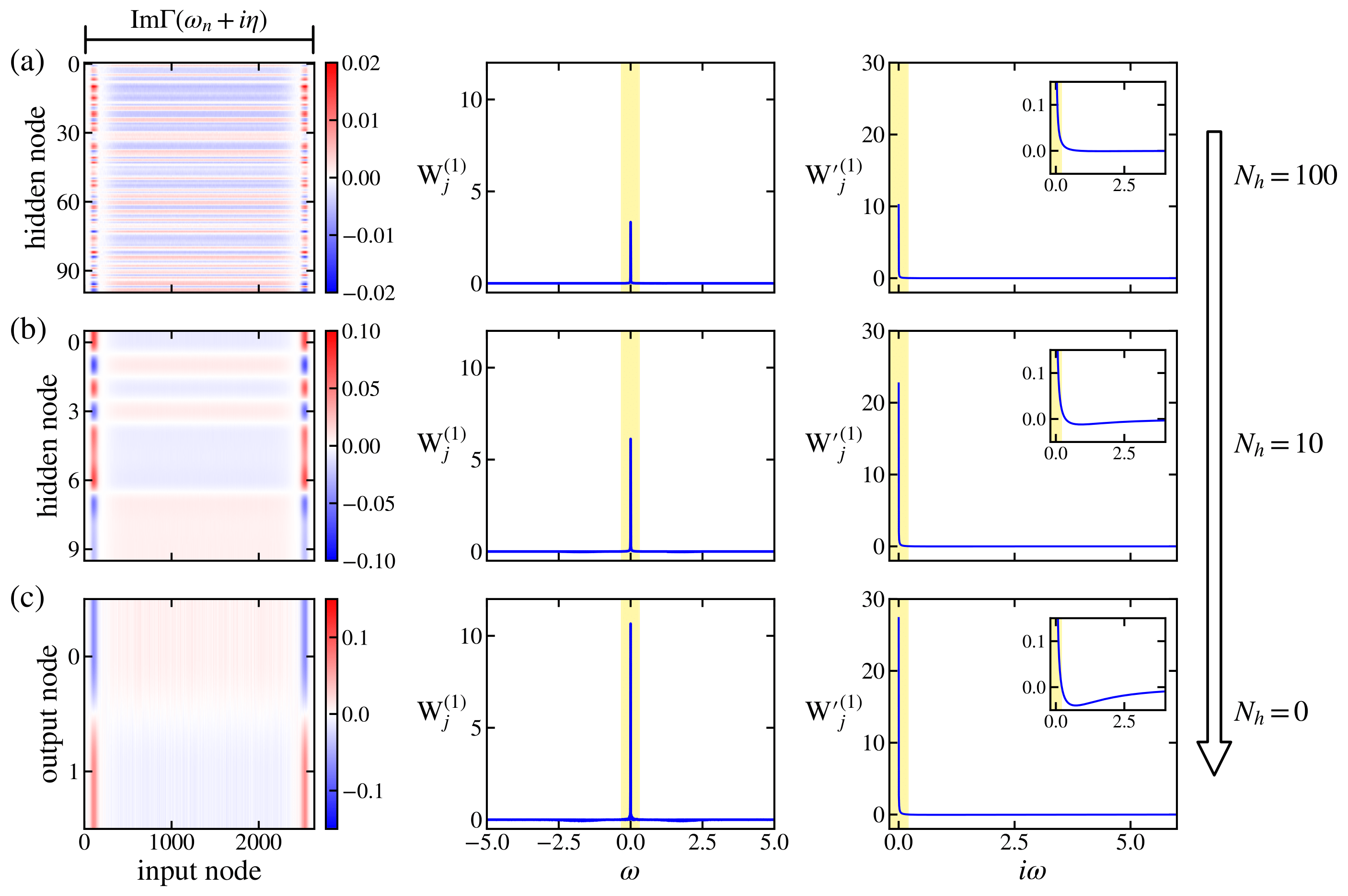
The comparable response of the weight matrix $\mathbf{W}^{(1)}$ of different models demonstrates that there are universal patterns of the dataset. The kernel density estimation~\cite{KDE} of the weight matrix $\mathbf{W}^{(1)}(\omega)$ on the real frequency axis exhibits these features, which is the high weight near the zero-frequency region in the imaginary part of the hybridization function. Surprisingly, the kernel density estimation of $\mathbf{W}^{\prime(1)}(i\omega_n)$ on the Matsubara frequency axis also displays the high weight near the zero-frequency region.

The analysis clarifies the consistency of network transformation as it preserves the significant patterns in the hybridization function $\Gamma(\omega)$ and $\Gamma(i\omega_n)$, which implies that the zero-frequency region manifests the connection between the different frequency domains.

Effective order parameter

Using the feature of the zero-frequency region on phase discrimination, we will mainly focus on the low-frequency region. Self-energy $\Sigma(i\omega_n)$ is given via the Dyson equation, \(\Sigma(i\omega_n) = i\omega_n + \mu - \sum_{k} \frac{V_k^2}{i\omega_n - \epsilon_k} - \frac{1}{4}\Bigg( \sum_{k}\frac{V_k^2}{i\omega_n - \epsilon_k} \Bigg)^{-1}\\ \text{Im} [\Sigma(i\omega_n)] = \omega_n + K(\omega_n) -\frac{1}{4}\Lambda(\omega_n)\\ K(\omega_n) = \sum_k{\bigg[\frac{\omega_n V_k^2}{\omega_n^2 + \epsilon_k^2} \bigg]} \\ \Lambda(\omega_n) = \frac{\sum_k{\frac{\omega_n V^2_k}{w^2_n+\epsilon^2_k}}}{\Big( \sum_{k}{\frac{ \omega_n V^2_k}{w^2_n + \epsilon^2_k}} \Big)^2 + \Big( \sum_{k}{\frac{\epsilon_k V^2_k}{w^2_n + \epsilon^2_k}}\Big)^2}\) Since $\text{Im}[\Sigma(i\omega_n)]=\sum_{p=-1}^{\infty}{A_p \omega_n^p}$, and comparing these two equations, \(\sum_{p=-1}^{\infty}{A_p \omega_n^p} = \omega_n + K(\omega_n) - \frac{S_2 \omega_n + O(\omega_n^3)}{4 \big( S_1^2 + \xi \omega_n^2 + O(\omega_n^4) \big)}\\ S_n = \sum_k{\bigg[ (1-\delta_{\epsilon_k, 0}) \frac{V_k^2}{\epsilon_k^n}\bigg]}, \\ M = \sum_k{\big[\delta_{\epsilon_k,0}V_k^2\big]}, \\ R = \sum_k{\big[ (1-\delta_{\epsilon_k,0})/\epsilon_k^2\big]}\) and thus \(A_{-1}=-\frac{S_2}{4(S_2+M)^2}\\ \text{Im}[\Sigma(i\omega_n)] \sim -\frac{S_2}{4 \big( S_2 + M \big)^2} \frac{1}{\omega_n}\) Previous studies shows \(A_{-1} = \bigg[ \int_{-\infty}^{\infty} d \omega_0 \frac{A(\omega_0)}{\omega_0^2}\bigg]^{-1}\) where $A_{-1}$ highly depends on zero-frequency region. We expect $A(w=\epsilon_k)\propto V_k^2$ by comparing above two equations, then we conclude that below equation is the integral representation of above equation.

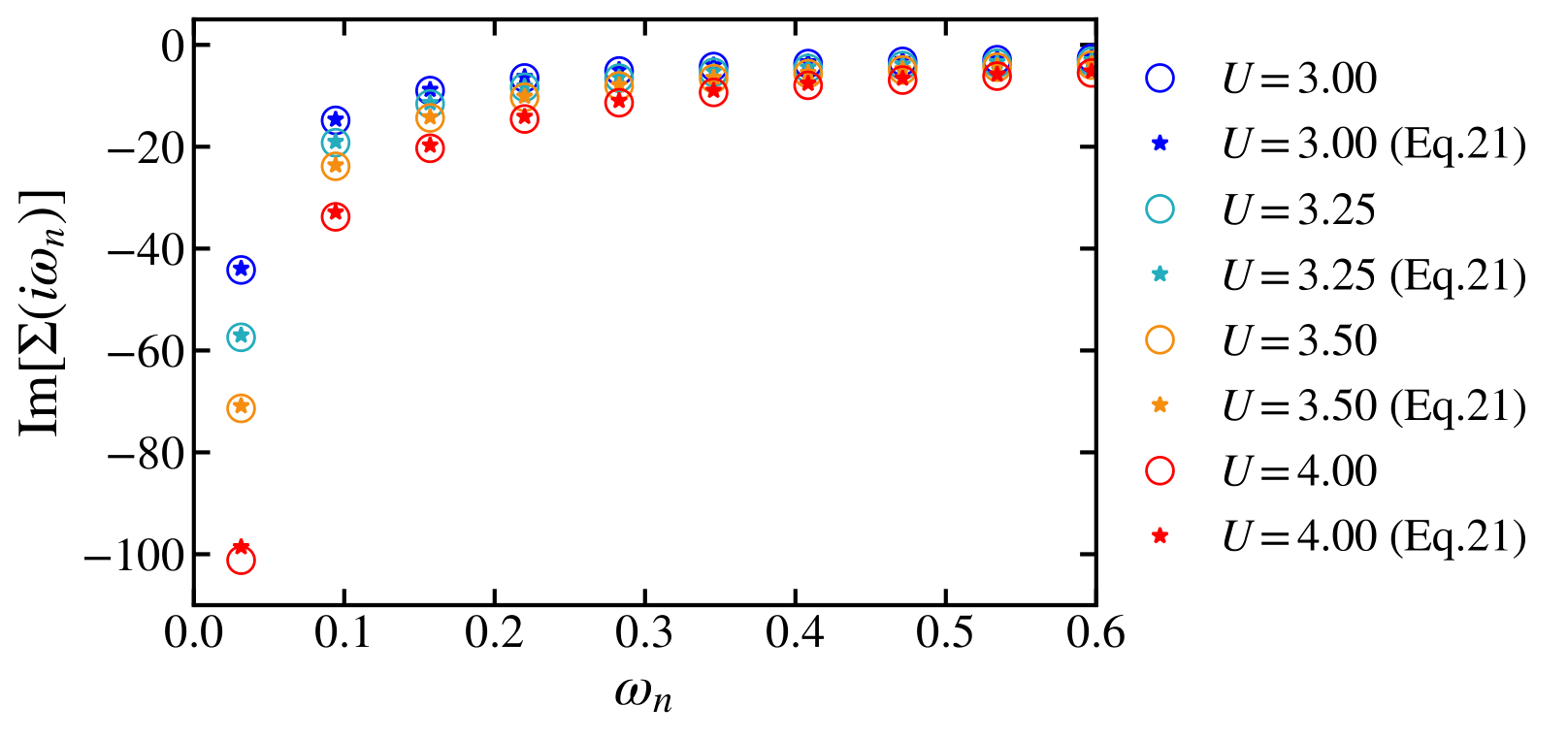
Above figure is for the imaginary part of the self-energy in the insulating phase for various $U$, and it shows that above equation agrees with the original datasets within numerical accuracy. Therefore, $S_2$ can be used to classify phase. Moreover, as $A_{-1}$ is not only related to bath parameters along with the Matsubara frequency domain, but also related the spectral function on the real frequency domain, $S_2$ provides the connection between the different frequency domain, and thus also provides the consistency of network transformation.

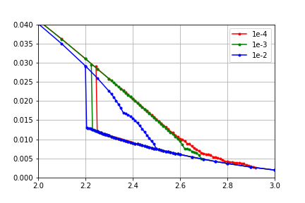
To verify whether the use of $S_2$ is valid in our case, we calculated $S_2^{-1}$ in different lattice geometries. $S_2^{-1}$ for the Bethe lattice changes steeply near the transition points. In the metallic phase, $S_2^{-1}$ is close to zero, as we expected. On the other hand, as $U$ increases in the insulating phase, $S_2^{-1}$ gradually increased as well. $S_2$ gives distinct values depending on the phase even within the phase coexistence region. Furthermore, to investigate the cases in different lattice geometries such as simple cubic(SC) and body-centered cubic(BCC) lattice where no clear evidence with analytical expressions for $S_2$. Figure below, which illustrates $S_2^{-1}$ for SC and BCC, also shows discontinuity near two transition points $U_{c1}$ and $U_{c2}$.

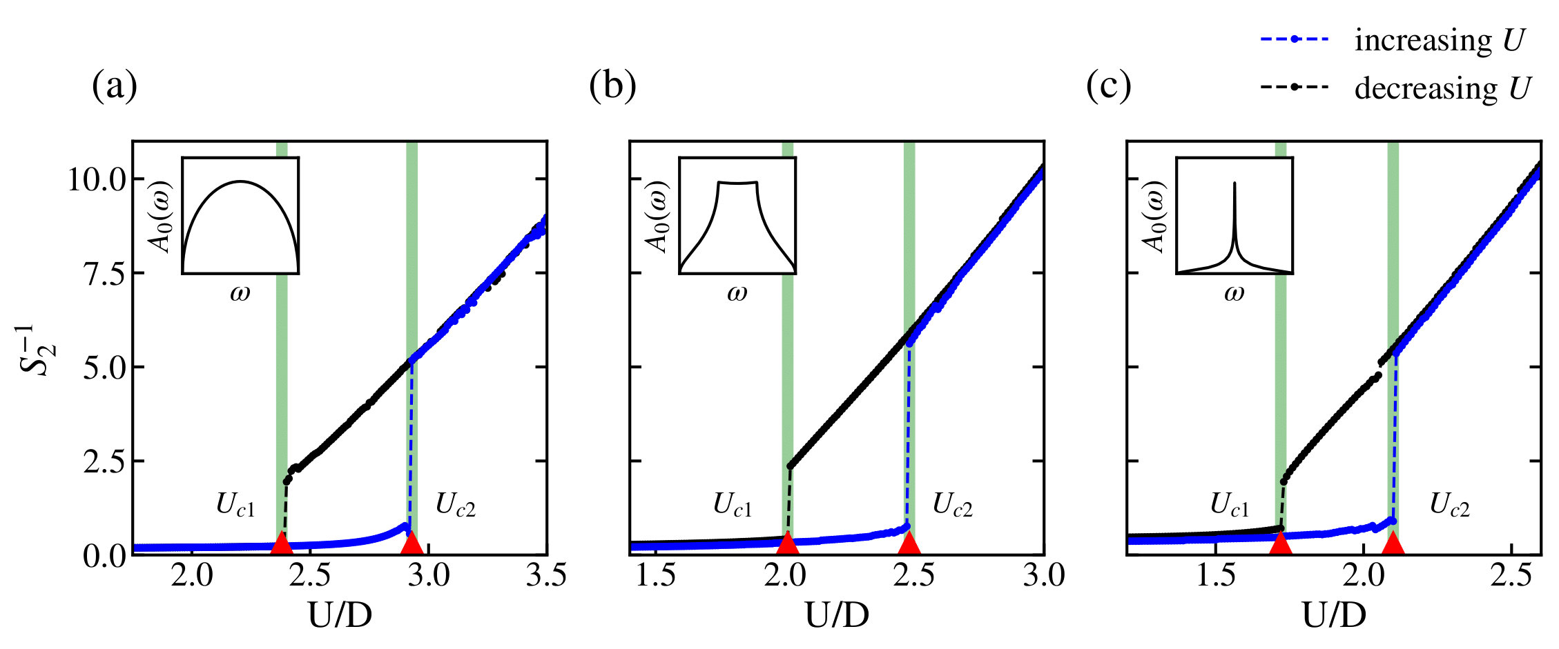
We conclude that $S_2$ excels in discriminating metallic-insulating phase regardless of the lattices structures, and therefore can be considered as an effective order parameter.

Summary

key topic: relationship between metal-insulator transition and the bath orbitals in the dynamical mean-field theory using explainable machine learning approaches.

Results:

1. Description of hamiltonian, self consistent equation, and DMFT-ED bath orbital projection. Explain the reason for using hybridization function first.
2. Train supervised machine learning with the hybridization function. Presents high accuracy regardless of the model complexity. Analyzing(=KDE) features of network parameter (=weight matrix), reveals that the model has high response on the imaginary part of the hybridization function, both on the real frequency and the Matsubara frequency. By low-frequency expansion of the hybridization function, we extracted some analytic expression from the zero-frequency region of the imaginary part of the hybridization function. Our neural network has extraced the pattern that reveals the relationship between the bath orbitals and the phases of matter.
3. Low frequency expansion of insular solution reveals some analytic expression which is consistent with the previous prediction of order parameter. For the insulating phase, this expression reduces to S2, which has very similar structure of what our neural network has extracted. We pose a hypothesis of new relationship between the bath parameters and the phase transition through S2. By calculating S2 in other lattices where no closed-form self-consistent equation exist, we verified that S2 is an effective order parameter. The low-frequency expansion of self-energy in terms of bath parameters also manifests the consistency with the atomic limit solution of the Hubbard model in the low-frequency regime.

Reference

1. https://en.wikipedia.org/wiki/Dynamical_mean-field_theory
2. A. Georges, G. Kotliar, W. Krauth, M. J. Rozenberg, Dynamical mean-field theory of strongly correlated fermion systems and the limit of infinite dimensions, Rev. Mod. Phys. 68, 13 (1996)
3. R. Bulla, T. A. Costi, D. Vollhardt, Numerical renormalization group method for quantum impurity systems , Rev. Mod. Phys. 80, 395 (2008)
4. E. Parzen, On Estimation of a Probability Density Function and Mode, Ann. Math. Stat. 33, 1065 (1962)