Interpretation of a minimal neural network to learn the metal-insulator transition in the dynamical mean-field theory

This work is a collaborative work.

In this research, we address the derivation of a new measure through interpretation of machine learning by employing DMFT with single-band Hubbard model which experiences a metal-insulator transition. Our goal is to present a machine learning scheme that detects the metal-insulator transition and to interpret the pattern of the neural network with respect to the phase of matter.

• Conducting DMFT-NRG and obtain data from it.
• Train neural network model with DMFT-NRG hybridization function, calculate accuracy.
• Interpretation of weight pattern of neural network connectivity.
• Derive a simple expression inspired by this interpretation.
• Investigate the performance of this phase indicator
• Discussion on the relationship between phase indicator and the quasiparticle weight.

Learning a metal-insulator transition from DMFT

DMFT procedure

Dynamic mean-field theory is the method to describe the properties of the strongly correlated materials. The Hamiltonian of the single orbital Hubbard model is \(H=-t\sum_{i,j,\sigma}{\bigg(c^{\dagger}_{i\sigma}c_{j\sigma}+c^{\dagger}_{j\sigma}c_{i\sigma}\bigg)+U\sum_{i}{n_{i\uparrow}n_{i\downarrow}}}+\mu\sum_{i\sigma}n_{i\sigma}\) where $\mu$ is the chemical potential, $t$ is the hopping element, and $U$ is the on-site interaction. The system experiences Mott transition by tuning $U$ in half-filling ($\mu=U/2$).

DMFT maps many-body lattice problem into the local problem, such as Anderson Impurity model (AIM).

\[H_\text{AIM} = \sum_k \epsilon_k a_k^\dagger a_k + \sum_{k\sigma}V_k^\sigma\bigg(c_\sigma^\dagger a_{k\sigma}+a_{k\sigma}^\dagger c_\sigma\bigg) + Un_\uparrow n_\downarrow - \mu(n_\uparrow+n_\downarrow)\]

where $\epsilon_k$ is the electronic level of the bath and $V_k$ is the hopping term between the impurity and the bath. Using the Anderson impurity model, it is now solvable with the self-consistency equation. (Various solvers are such as NRG(numerical renormalization group), ED(exact diagonalization), or QMC(quantum Monte-Carlo).) One DMFT loop consists of the following steps.

1. DMFT mapping onto AIM.
2. Solve AIM with specific solver.
3. Extract self-energy of the impurity mode, make DMFT approximation on lattice self-energy.
4. Repeat.

DMFT-NRG is the method that can calculate the exact spectral function on the real frequency without analytic continuation. This method is capable of calculating on the arbitrary low temperature scale using the renormalization group techniques by employing logarithmic intervals. (Vast majority of the data is centered near zero frequency.)

In Bethe lattice, self consistency: $\Gamma = D^2 G/4$. Implementing broyden method with hybridization function have increased the speed of calculation. \(\Gamma_{out} = dmftstep(\Gamma_{in}))\\ 0 = F(\Gamma_{new}) = dmftstep(\Gamma_{in})-\Gamma_{in}\)

Finally, calculated phase transition points $U_{c1}\sim2.3$ and $U_{c2}\sim2.9$. (See Previous work)

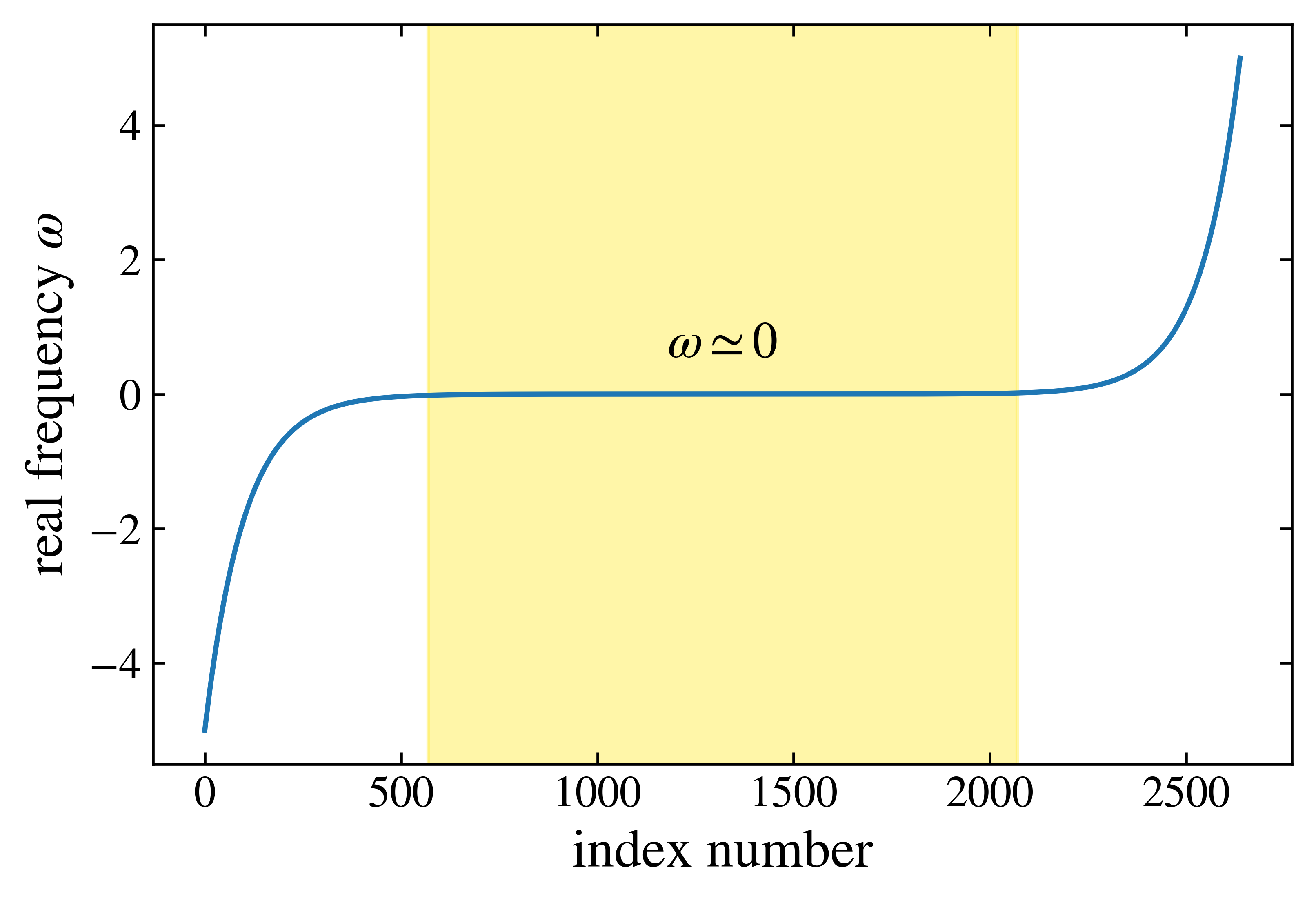
During DMFT procedure, hybridization function is used for reproducing lattice dynamics, as it is closely related to the dynamics of the electrons and the bath of the impurity by bath parameters. We calculated the hybridization function under logarithmic discretization mesh~(frequency) ratio of $\lambda=1.01$ spanning from $|\omega|=10^{-5}\sim5.0$. For the NRG calculation parameters, we set logarithmic discretization parameter $\Lambda=2.0$, the number of interleaved discretization grids $N_z=4$, the lowest temperature scale of Wilson chain $T_{min}=10^{-6}$, and the truncated rescale energy cutoff $12.0$ for the good convergence.

Artificial neural network to learn the spectral features

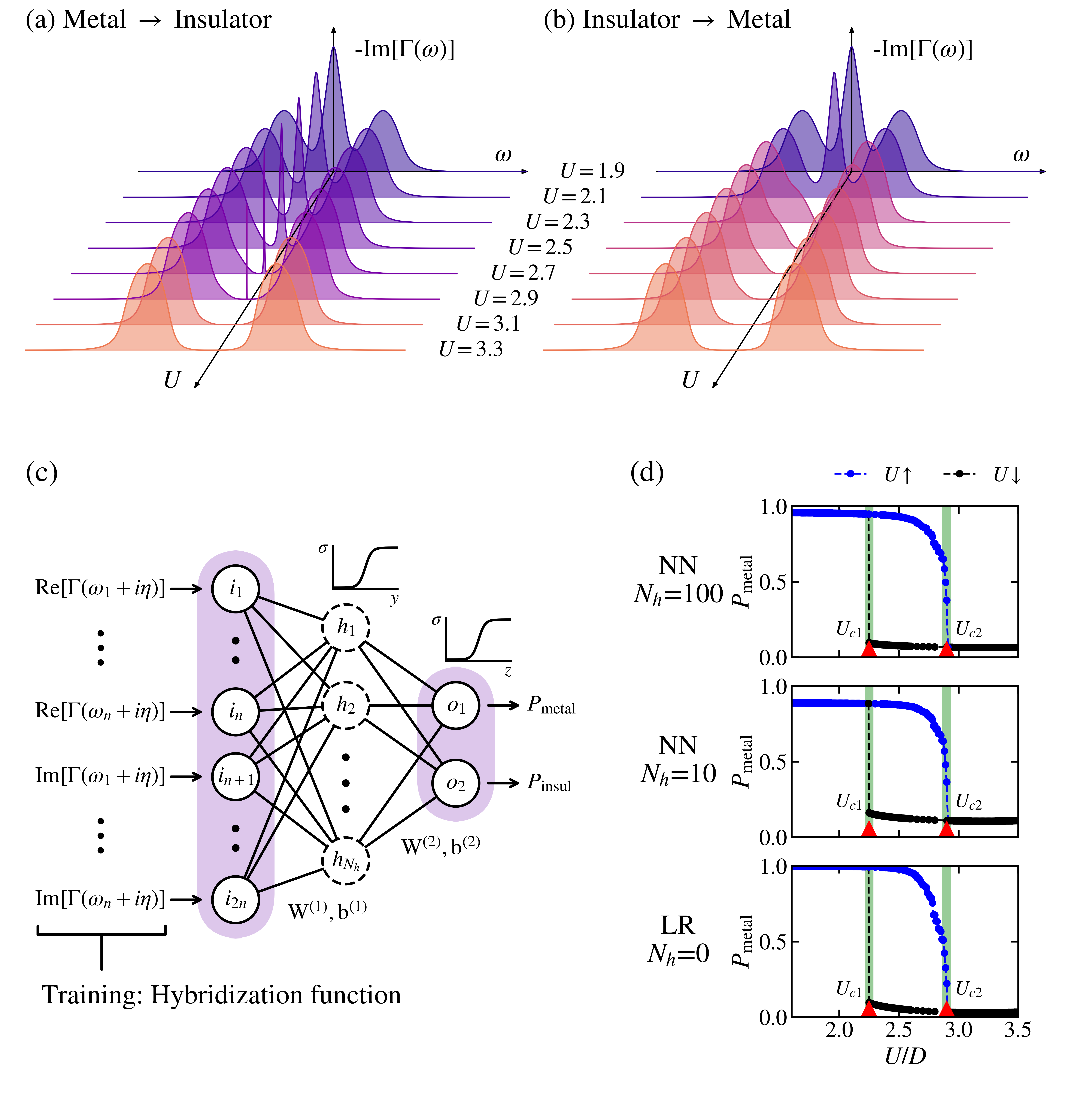
The scheme of supervised machine learning model that classifes phase based on the hybridization is illustrated above. The neural network receives the hybridization function $\Gamma(\omega_n)$ as an input, and gives the probability of being in each phase as an output. The sigmoid function $\sigma(x) = 1/(1+\exp(-x))$ is employed as an activation function between each layer.

\(\mathbf{y}=\mathbf{W}^{(1)}\Gamma(\omega_n)^{\mathbf{T}} + \mathbf{b}^{(1)}, \\ \mathbf{z}=\mathbf{W}^{(2)}\sigma(\mathbf{y})+ \mathbf{b}^{(2)}, \\ \mathbf{P}=\sigma(\mathbf{z}),\) where each $\mathbf{W}^{(i)}$ and $\mathbf{b}^{(i)}$ are the weight matrix and the bias vector, and $\mathbf{P}$ is the output vector of our model which is $\mathbf{P}=(P_\text{metal},P_\text{insulator})^\mathbf{T}$.

The neural network is trained with the hybridization function on the real frequency axis obtained by DMFT-NRG. The training set consists of the data in the Bethe lattice under half-filling for a given range of on-site interactions of metallic phase $U_M^{(tr)}={u \mid 0.5\leq u\leq 2.0}$ and of insulating phase $U_I^{(tr)}={u \mid 3.0\leq u\leq 5.0}$. By excluding region around phase coexistence $U={u \mid U_{c1} \leq u \leq U_{c2}}$ from the training set, we can examine whether our machine representation can be extended to the phase coexistence region.

The testing set consists of the data in the same condition as the training set but for the range of on-site interactions including phase coexistence region $U={u \mid U_{c1} \leq u \leq U_{c2}}$. This corresponding test output in Fig (d) demonstrates that our neural network models have a high accuracy of predicting transition points $U_{c1}$ and $U_{c2}$ by reconstructing the discontinuous hysteresis behavior of the first-order phase transition. Even without the hidden layer, the logistic regression model output shows the high accuracy of classification of each phase within the phase coexistence region. The high accuracy regardless of the model complexity also implies that our models have converged to the same solution.

Extracting a simple phase indicator

Figure below displays the heat map of the weight matrix $\mathbf{W}^{(1)}$ of different models in order of decreasing complexity. This pattern shows a similar weight response toward the real and the imaginary part of the hybridization function regardless of the model kind, roughly divided into low and high-frequency regions.

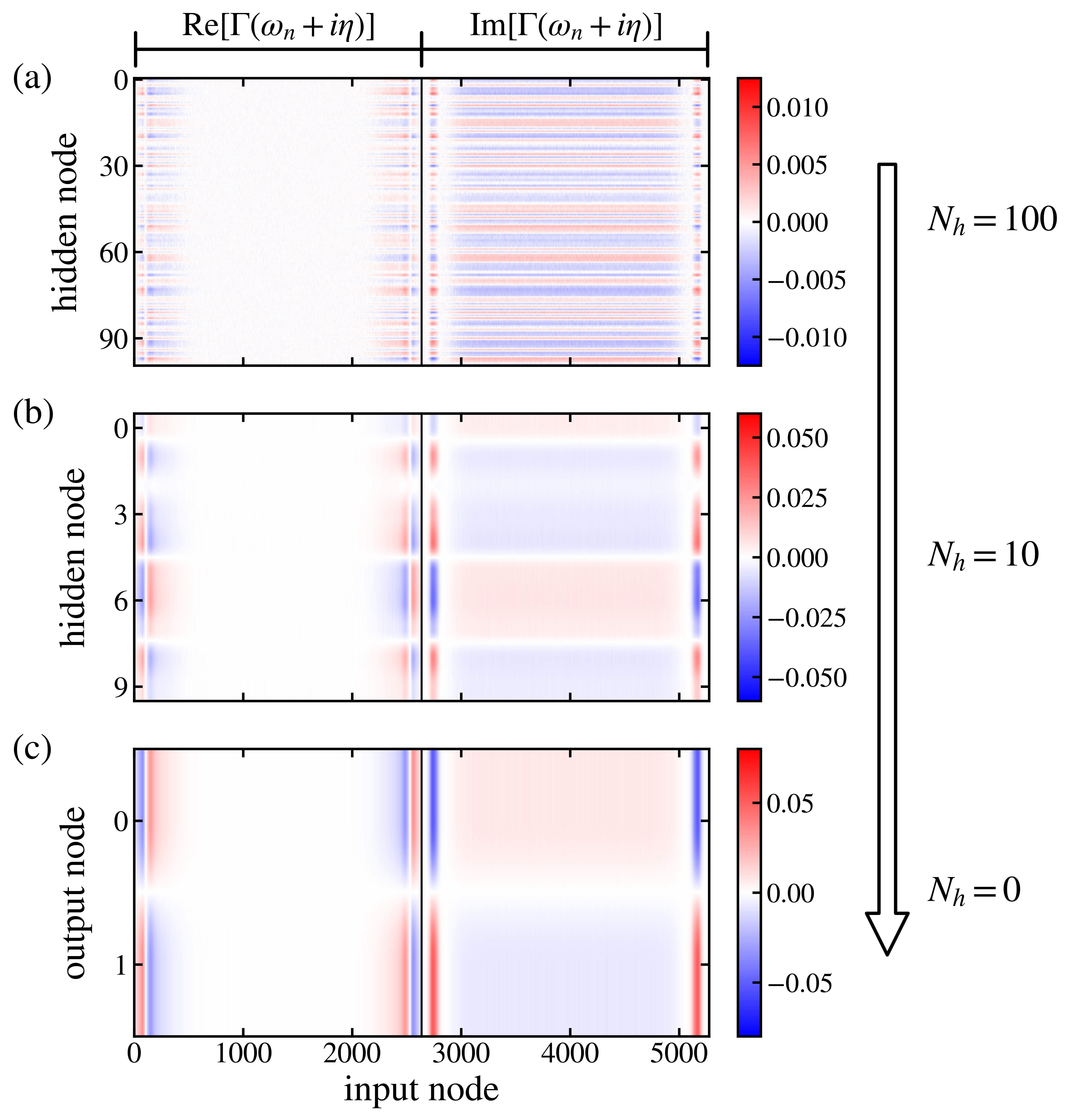
Regarding this universality of weight patterns, we choose to investigate the Logistic regression model to understand this general pattern. Considering the density of data $\rho(\omega) = 1/|\omega|$ due to logarithmic discretization $|\omega_n|\sim\lambda^{-n}$ and the hybridization function $\Gamma(\omega+i\eta) = \sum_kV_k^2/(\omega+i\eta-\epsilon_k)$ with respect to the bath parameters in DMFT-ED, output $\mathcal{O}$ of the regression on the real frequency domain is \(\begin{aligned} \mathcal{O} &= \sum_n \left[\mathbf{W}^{(1)}_{Re, n}\text{Re}\left[\Gamma(\omega_n)\right] + \mathbf{W}^{(1)}_{Im, n}\text{Im}\left[\Gamma(\omega_n)\right]\right]\\ &\simeq \int d\omega\rho(\omega)\mathbf{W}^{(1)}_\text{Re}(\omega)\text{Re}\left[\Gamma(\omega+i\eta)\right] + \int d\omega\rho(\omega)\mathbf{W}^{(1)}_\text{Im}(\omega)\text{Im}\left[\Gamma(\omega+i\eta)\right]\\ &= \int\frac{d\omega}{|\omega|}\mathbf{W}^{(1)}_\text{Re}(\omega)\sum_k\frac{V_k^2}{\omega-\epsilon_k} + \int\frac{d\omega}{|\omega|}\mathbf{W}^{(1)}_\text{Im}(\omega)\sum_kV_k^2\delta(\omega-\epsilon_k), \end{aligned}\)

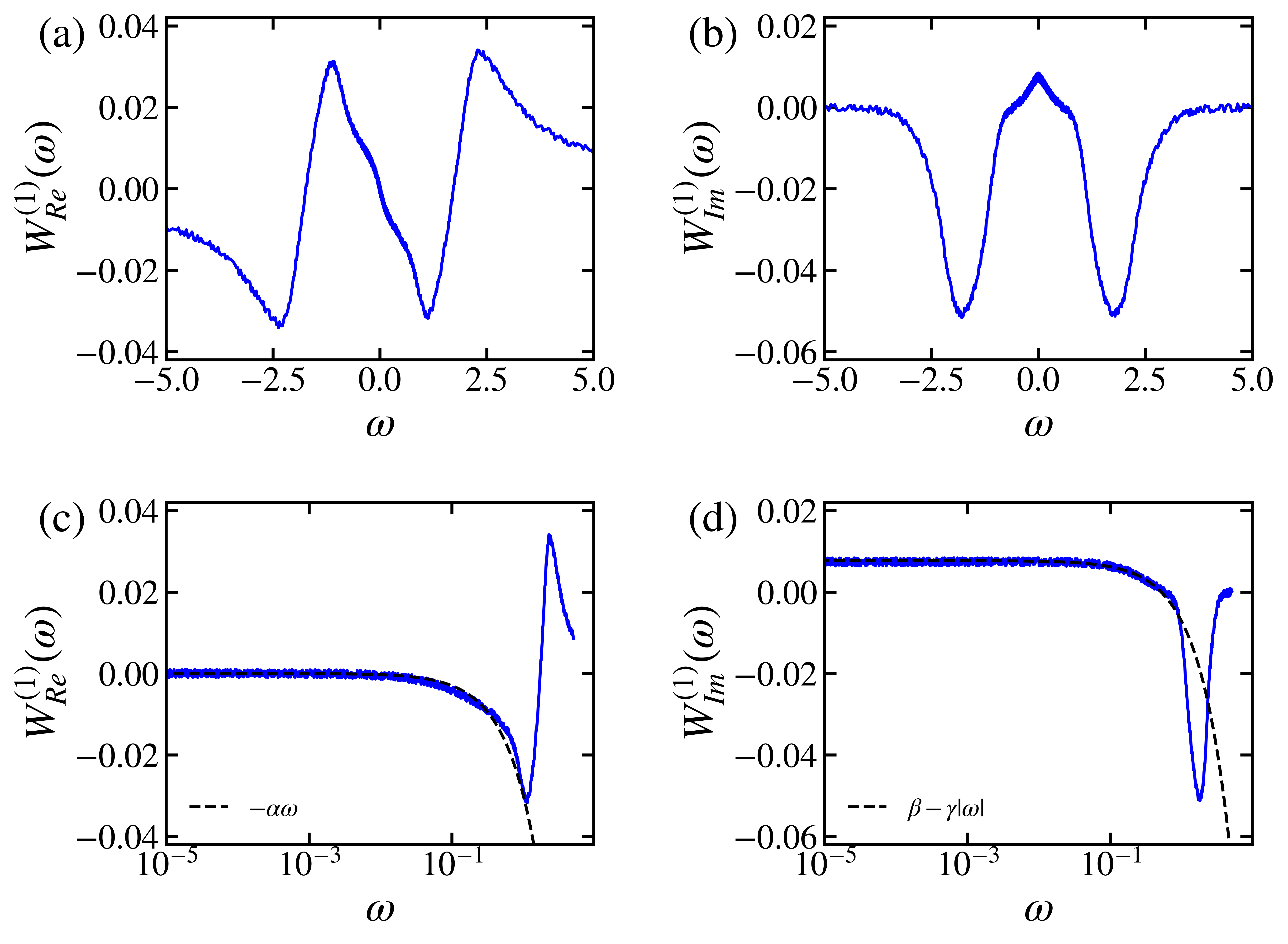
Above figure presents the behavior of the weight matrix of the Logistic regression corresponding for the real and the imaginary part of the hybridization function. We aim to look into the vicinity of the zero frequency $\omega\simeq0$ due to the concentration of data near this point. Along with the simple polynomial fitting for each matrix, the analysis exhibits $\mathbf{W_{Re}}^{(1)}\sim-\alpha\omega$ and $\mathbf{W_{Im}}^{(1)}\sim\beta-\gamma|\omega|$ on low frequency regime for positive real number $\alpha\approx3.5\times10^{-2}$, $\beta\approx7.7\times10^{-3}$ and $\gamma\approx1.5\times10^{-2}$. Substituting this weight matrix behavioral information, equation becomes \(\begin{aligned} \mathcal{O}&\simeq \int\frac{ d\omega}{|\omega|}(-\alpha\omega)\sum_k\frac{V_k^2}{\omega-\epsilon_k} + \int\frac{ d\omega}{|\omega|}(\beta-\gamma|\omega|)\sum_kV_k^2\delta(\omega-\epsilon_k)\\ &= -2\alpha\sum_k\int_{|\omega|_{\text{min}}}^{|\omega|_{\text{max}}}\frac{V_k^2}{\omega+|\epsilon_k|} d\omega + \beta\sum_k\frac{V_k^2}{|\epsilon_k|}-\gamma\sum_kV_k^2\\ &= -2\alpha\sum_k V_k^2\log\left(1+\frac{|\omega|_{\text{max}}-|\omega|_{\text{min}}}{|\epsilon_k|+|\omega_{\text{min}}|}\right) + \beta\sum_k\frac{V_k^2}{|\epsilon_k|}-\gamma\sum_kV_k^2\\ &\simeq 2\alpha\sum_k V_k^2\log(|\epsilon_k|) + \beta\sum_k\frac{V_k^2}{|\epsilon_k|}-(\gamma+2\alpha\log(|\omega|_{\text{max}}-|\omega|_{\text{min}}))\sum_kV_k^2, \end{aligned}\) where the last term is constant by the sum-rule of hopping elements $V_k$ of our neural network.

Performance of the machine-learning-inspired phase indicator

We examine the above equation based on the discrete model of few bath orbitals calculated by DMFT-ED, to figure out what our analysis indicates.

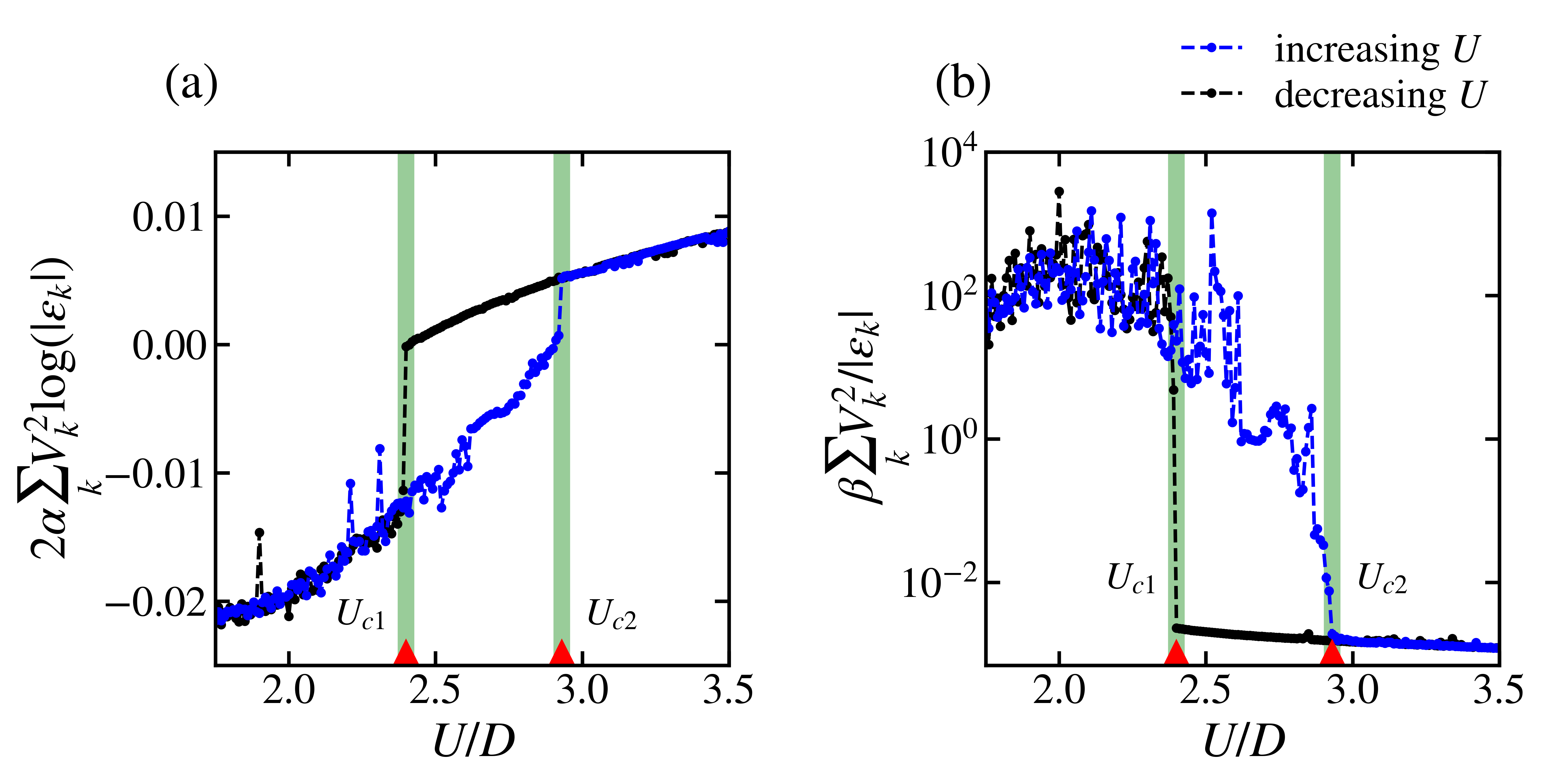
Figure above shows the usage of two terms $2\alpha\sum_kV_k^2\log(\mid\epsilon_k\mid)$ and $\beta\sum_kV_k^2/\mid\epsilon_k\mid$ results in the phase discrimination, which shows a clear discontinuity near two transition points $U_{c1}$ and $U_{c2}$. The result demonstrates that two terms $\sum_kV_k^2\log(\mid\epsilon_k\mid)$ and $\sum_kV_k^2/\mid\epsilon_k\mid$ are capable of classifying the phase between metallic phase and insulating phase with minor numerical error. Surprisingly, we found that the latter term $\sum_kV_k^2/\mid\epsilon_k\mid$ dominates in our neural network output by comparing two phase diagrams. Therefore we conclude that the neural network classifies phase based on the imaginary part of the zero-frequency hybridization function. We also suggest a new relationship between the bath parameters and the phase classification by means of $\sum_kV_k^2/\mid\epsilon_k\mid$, which we will denote this as $S$.

To verify our hypothesis, we calculated $S^{-1}$ based on few bath parameters for various on-site interaction $U$.

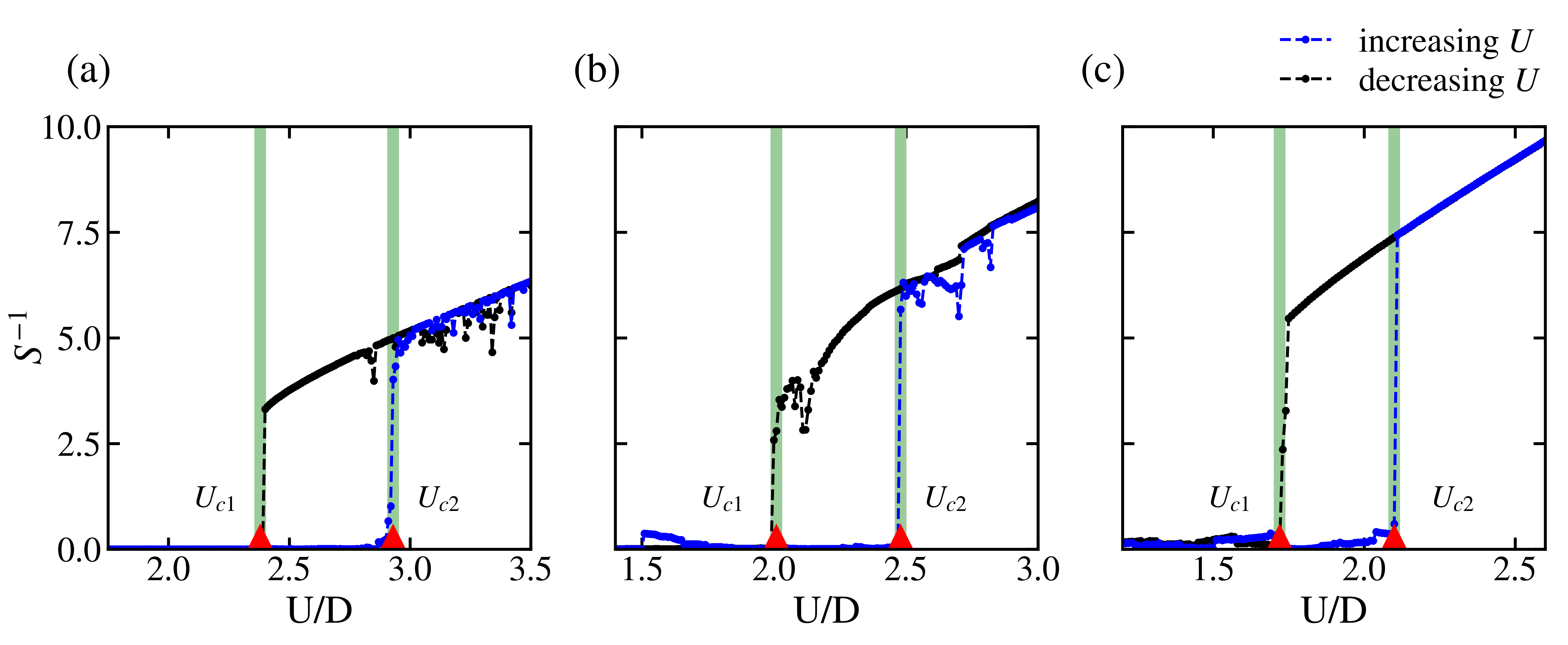
Presented in above figure, $S^{-1}$ for the Bethe lattice changes steeply near the transition points $U_{c1}$ and $U_{c2}$. In the metallic phase, $S^{-1}$ is close to zero as $S$ diverges to infinity. For the case where $U$ increases in the insulating phase, $S^{-1}$ gradually increases as well. To sum up, $S^{-1}$ gives distinct values depending on the phase. Furthermore, to investigate the cases in different lattice geometries, we apply $S^{-1}$ to other lattices such as simple cubic (SC) and body-centered cubic (BCC) lattice. We examine whether $S^{-1}$ also appears as the critical feature of discriminating a phase even in SC and BCC lattices by numerical means. As a result, Fig.~\ref{fig:phaseall}~(b,c), which illustrates $S^{-1}$ for SC and BCC lattices each, also shows discontinuity near two transition points $U_{c1}$ and $U_{c2}$. We conclude that $S^{-1}$ works well for discriminating metallic-insulating phase regardless of the lattices structures and therefore can be considered as a phase discriminator.

Discussion