Quantum Ising model

This page is for the summary of my presentation on course “Thermal & Statistical Physics”. Actual presentation in here.

Classical Ising model

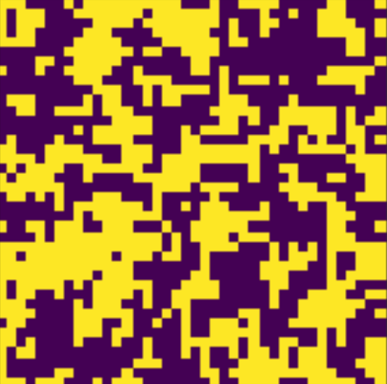
For the simplest Ising model for spin-1/2, the energy configuration is given by Hamiltonian. \(H = -J\sum_{<i,j>} s_is_j- B\sum_i s_i\) This model is the simplest model of a magnet. $J$ indicates the interaction between nearest neighbors. It is ferromagnetic for $J>0$ and $B$ stands for external magnetic field. Ising model experiences second-order phase transition.

Mean field theory for $d$-dimensional lattice

By using Mean field approximation we can determine the solution for d-dimension system. Our goal is to discover partition function.

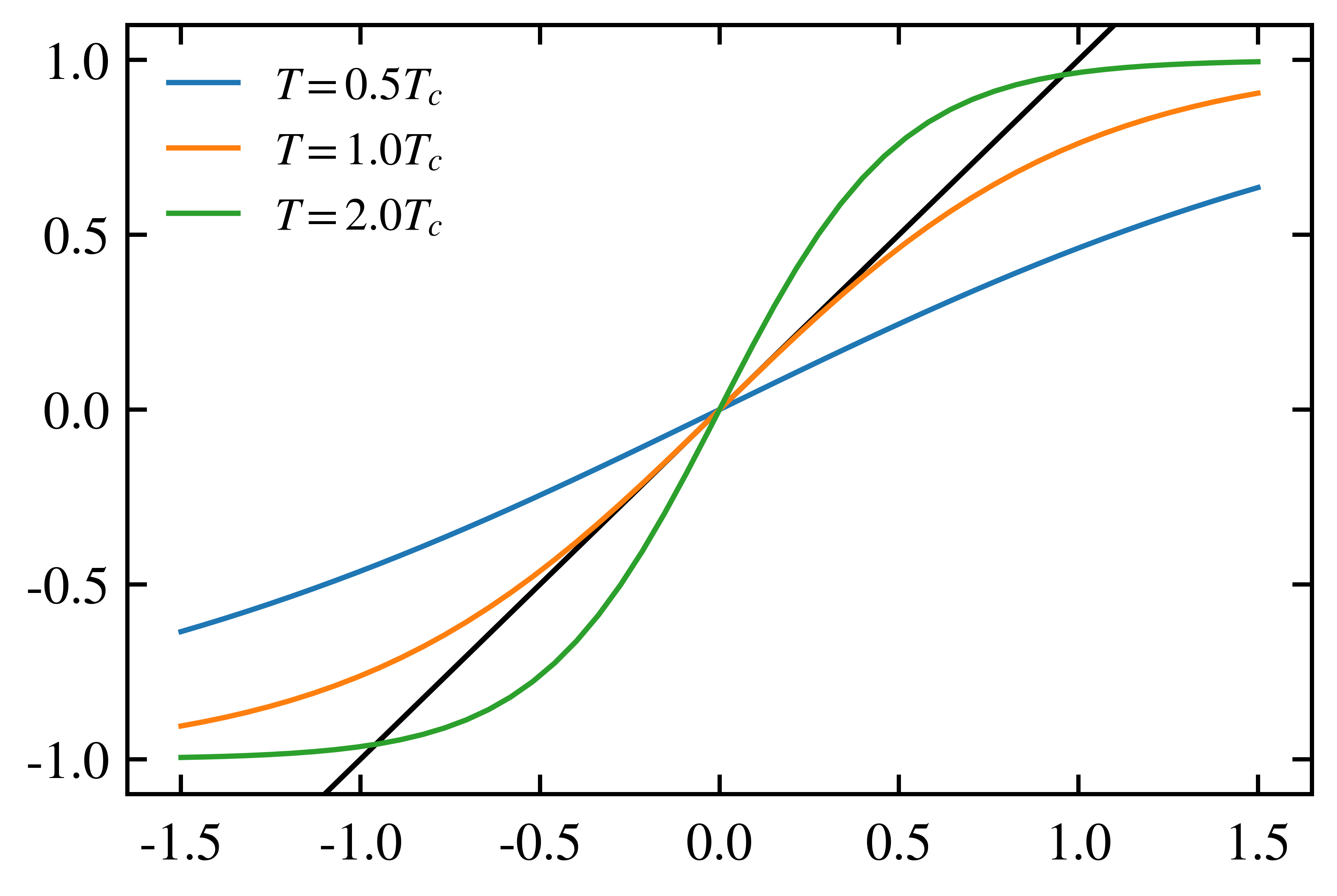
First, let $s_i = \langle s\rangle+\delta s_i, \; s_j = \langle s\rangle +\delta s_j$, and put into Hamiltonian. $z$ implies number of nearest neighbors in the lattice. \(\begin{aligned} H =& -J\textstyle\sum_{\langle i,j\rangle}s_is_j - B\sum_i s_i \\=& -J\sum(\langle s\rangle+\delta s_i)(\langle s\rangle+\delta s_j)-B\sum s_i \\=& -\frac{1}{2}zJ\textstyle\sum_i\langle s\rangle s_i-B\sum s_i + const. \\Z =& \sum_{\{\vec{s}\}}\prod_i^N\exp\left(\tfrac{1}{2}\beta z J\langle s\rangle s_i+\beta B s_i\right) \\=& 2^N\cosh^N\left(\tfrac{1}{2}\beta z J\langle s\rangle +\beta B\right) \\ \therefore\;\langle s\rangle =& -\frac{1}{N\beta}\frac{\partial \ln Z}{\partial B} = \tanh(1/2\,\beta zJ\langle s\rangle +\beta B)\quad\Rightarrow T_c = z/2 \end{aligned}\)

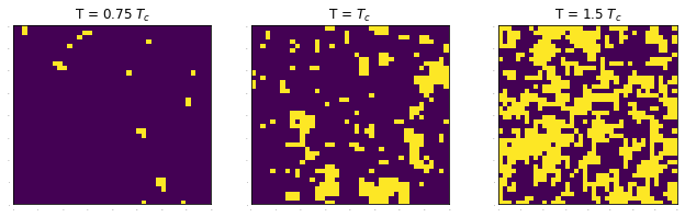
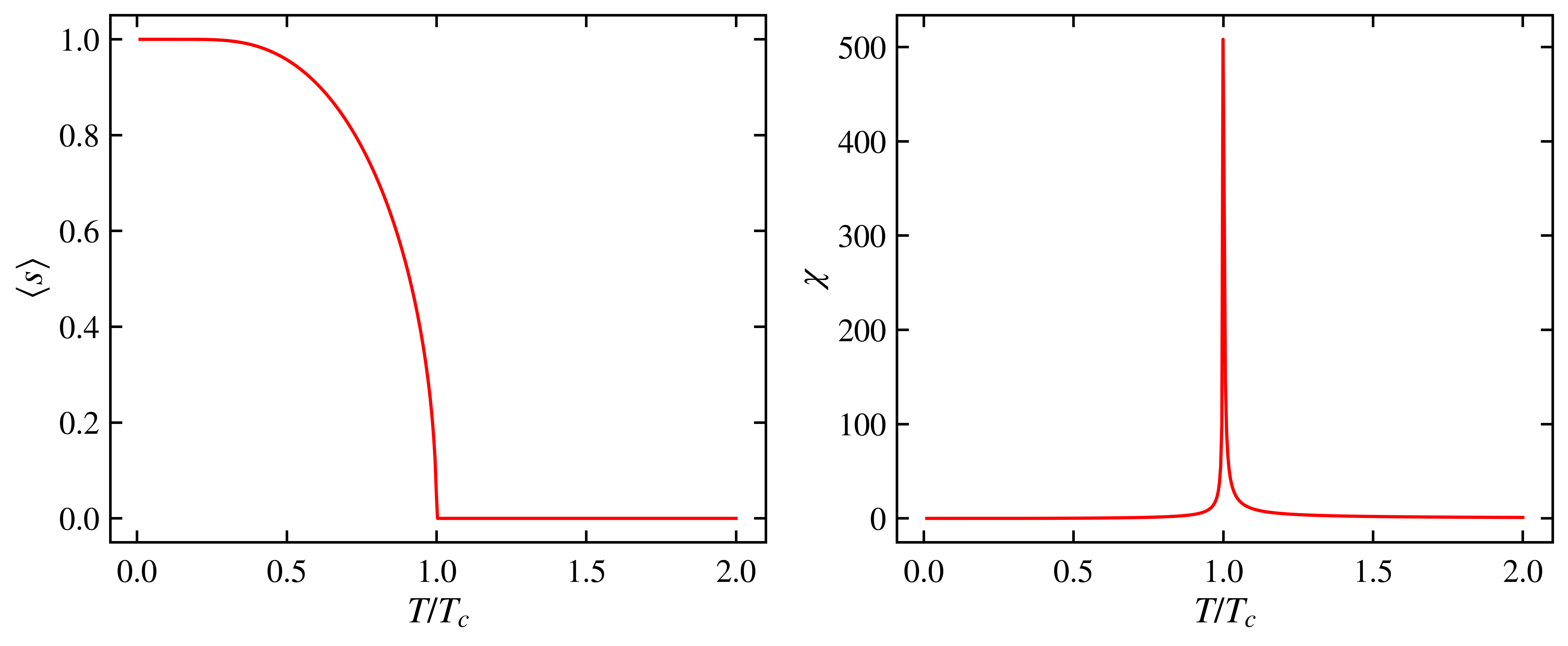
Now we figured out the mean value of spin, in other words, magnetization. Large $\beta$ with small temperature will have 2 non-zero stable point and 1 unstable point $\langle s\rangle=0$. For large temperature, only 1 stable point at magnetization 0, the disordered phase.

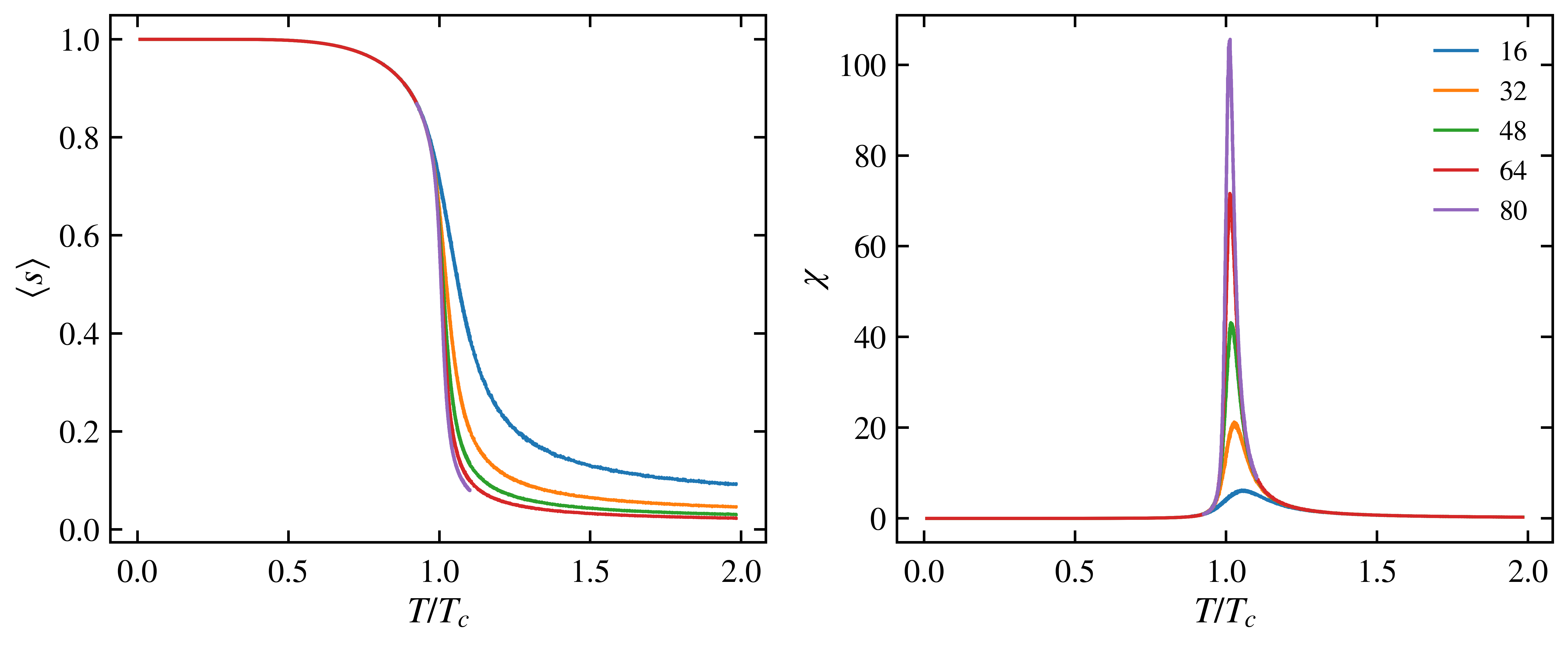
We can also determine the critical point where phase transition occurs, but it is quite incorrect for small dimensions.

These are the simulated results using Mean field theory.

Transverse field Ising model

Transverse field Ising model is quantum version of classical Ising model. This system is determined by alignment of spin projections along $z$-direction, as well as external magnetic field perpendicular to $z$-direction (along $x$-direction, we may think), creates bias for $x$-direction spin. \(\mathcal{H} = -J\left(\sum_{\langle i,j\rangle}Z_iZ_j+g\sum_jX_j\right)\) Here, $X, Z$ are spin algebras. (For spin-1/2 case, it is Pauli matrices, obviously.)

Correspondence with classical Ising model

Surprisingly, mapping between $d$-dimension quantum Ising model and $d+1$-dimension classical Ising model exists. How can this happen?

The main idea is this: Evaluating quantum Ising model partition function using $\delta t$, Imaginary time path integral. This is basically considering d+1 dimension classical Ising model as the time propagation of d-dimensional quantum Ising model.

1D classical Ising with 0D quantum Ising

First, we consider classical Ising model with periodic boundaries, which is same as chain in above figure. \(\mathcal{H}_c = -K\sum_{l=1}^M s_ls_{l+1} - h\sum_{l=1}^Ms_l\quad (K = J/\beta, h = B/\beta)\\ Z_c = \sum_{\{s_l = \pm1\}}e^{-\mathcal{H}_c} = \sum_{\{s_l\}}\prod_{l=1}^M e^{ks_ls_{l+1}}e^{hs_l} = \sum_{\{s_l\}}\prod_{l=1}^M T_1(s_l,s_{l+1})T_2(s_l)\\ T_1(s,s') = \begin{pmatrix}e^k&e^{-k}\\e^{-k}&e^k\end{pmatrix}_{ss'} = \langle s|\hat{T}_1|s'\rangle\\ \delta_{ss'}T_2(s) = \begin{pmatrix}e^h&0\\0&e^h\end{pmatrix}_{ss'} = \langle s|\hat{T}_2|s'\rangle\)

which this matrix element of operator $\hat{T}_1, \hat{T}2$ just like acting on 2-state quantum system. In other words, single quantum-spin of 2-states!

\(Z_c = \sum_{\{s_l\}}\langle s_1|\hat{T}_1\hat{T}_2|s_2\rangle\cdots\langle s_M|\hat{T}_1\hat{T}_2|s_1\rangle = \mathrm{tr} \\ (\hat{T}^M)= \lambda_+^M+\lambda_-^M\quad(\hat{T} = \hat{T}_2^{1/2}\hat{T}_1\hat{T}_2^{1/2}) \\ \lambda_\pm = e^k\cosh h \pm \sqrt{e^{2k}\sinh^2h+e^{-2k}}\to\begin{cases}2\cosh k\\2\sinh k\end{cases} \text{ when }h\to0\) $\hat{T}$ stands for transfer matrix. If we consider this operator as a propagator in time with spin-1/2, and assuming $\delta t\ll E_0^{-1}, h^{-1}$, \(\begin{aligned} \hat{T}_1\hat{T}_2 &= e^{b\mathbb{I}+a\hat{X}}e^{h\hat{Z}} = e^{-\hat{H}\delta t}\quad(\mathbb{I} = \sum_{s_i}|s_i\rangle\langle s_i|) \\\langle s_l|e^{b\mathbb{I}+a\hat{X}}|s_{l+1}\rangle &= e^b\begin{pmatrix}\cosh a&\sinh a\\\sinh a&\cosh a\end{pmatrix}_{s_ls_{l+1}} \\ &= \begin{pmatrix}e^k&e^{-k}\\e^{-k}&e^k\end{pmatrix}_{s_ls_{l+1}} = \langle s_l|\hat{T}_1|s_{l+1}\rangle \\ \therefore\;& e^{-2K} = \tanh a \\ \therefore\;& \hat{H} = -\frac{b}{\delta t}-\frac{a}{\delta t}\hat{X}-\frac{h}{\delta t}\hat{Z} = E_0 - \frac{\Delta}{2}\hat{X} - \bar{h}\hat{Z} \end{aligned}\) Let’s consider $\bar{h}=0$ for a moment, then $\Delta$ is the energy gap between groundstate and first excited state. Then the thermal partition function is \(Z_q = \mathrm{tr}(e^{-\beta\hat{H}}) = \sum_{\{s\}}\langle s|e^{-\beta\hat{H}}|s\rangle \quad\text{ in }\hat{Z} \text{ basis},\\ = \sum_{s_1,\cdots s_M}\langle s_M|e^{-\hat{H}\delta t}|s_{M-1}\rangle\cdots\langle s_1|e^{-\hat{H}\delta t}|s_M\rangle\\ \therefore \; e^{-2K} = \tanh \frac{\beta\Delta}{2M}\) $\beta=1/T$ as length of euclidean time circle that makes $\delta t = \beta/M$. The right-hand-side is the partition function of classical Ising chain, $K$ given by the last equation. Therefore, we conclude that there exist mapping between classical and quantum version of Ising model.

2D classical Ising with 1D quantum Ising

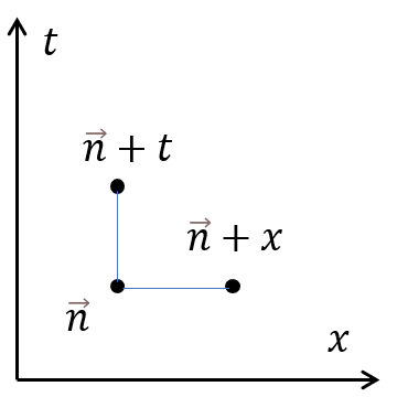
Next, we consider the classical case with more than one dimension. We basically do the same thing as before, but we consider one of the lattice direction as euclidean time. Then rewrite the classical Hamiltonian as \(H_c = -\sum_{\vec{n}}\left(Ks(\vec{n}+t)s(\vec{n})+K_x s(\vec{n}+x)s(\vec{n})\right)\\ =K\sum_{\vec{n}}\left(\frac{1}{2}(s(\vec{n}+t)-s(\vec{n}))^2-1\right)-K_x\sum_{\vec{n}}s(\vec{n}+x)s(\vec{n}) \\= \sum_{t=const, l}L(l+1, l) + const.\)

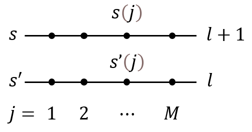
We define the Lagrangian $L(s, s’)$ with successive time slices named $s, s’$. Figure above describes this situation. \(L(s, s') = \frac{1}{2}K\sum_j(s(j)-s'(j))^2 - \frac{1}{2}K_x\sum_j(s(j+1)s(j)+s'(j+1)s'(j))\) The transfer matrix between successive time slices is $M(2^M)$ matrix. \(\langle s|\hat{T}|s'\rangle = T_{ss'} = e^{-L(s,s')}\\ Z = \sum_{\{s\}}e^{-H_c} = \sum_{\{s\}}\prod_{l=1}^M T_{s(l,j),s(l+1,j)} = \mathrm{tr}_\mathbb{H}\hat{T}^M\) This is just as in one-site case, but the difference is that Hilbert space $\mathbb{H}$ has two-state system for every site on fixed-$l$ (or fixed time) slice of lattice, or in other words, space. $\mathbb{H} = \otimes_j\mathbb{H}_j$.

Now, what we have to do is to estimate transfer matrix. The diagonal entries come from $s=s’$. \(L(0\text{ flip}) =-K_x\sum_js(j+1)s(j)\) The one-off diagonal term is from $s=s’$ except one $j$ with $s(j)=-s’(j)$. \(L(1\text{ flip}) = \frac{1}{2}K(1-(-1))^2-\frac{1}{2}K_x\sum_j(s(j+1)s(j)+s'(j+1)s'(j))\\ L(n\text{ flip}) = 2nK - \frac{1}{2}K_x\sum_j(\cdots)\) Now we can determine transfer matrix using \(\hat{T} = e^{-\hat{H}\delta t}\simeq1-\hat{H}\delta t\\ T(0\text{ flip})_{ss'} =\delta_{ss'}e^{K_x\sum_j(\cdots)}\simeq \mathbb{I}-\hat{H}(0\text{ flip})\delta t\\ T(1\text{ flip})_{ss'} =e^{-2K}e^{1/2K_x\sum_j(\cdots)}\simeq -\hat{H}(1\text{ flip})\delta t\\ T(n\text{ flip})_{ss'} =e^{-2nK}e^{1/2K_x\sum_j(\cdots)}\simeq -\hat{H}(n\text{ flip})\delta t\) To make time $t$ continuous, we assume $K\to \infty$ and $K_x\to 0$. (This is because $\delta t$ depends on coupling constant.)

Then we see that matrix element with $n$-flip goes like $e^{-nK}\sim(\delta t)^n$ which is very small, therefore, the Hamiltonian only contains 0 and 1-flip terms. Therefore, \(\hat{H} = -J\left(\sum_j\hat{Z}_j\hat{Z}_{j+1}+g\sum_j\hat{X}_j\right)\) where first term is from 0-flip, second term is from 1-flip case, and $g = e^{-2K}/K_x$. This whole Hamiltonian describes 1-dimensional transverse field Ising model.

$d+1$-dimensional classical Ising with $d$-dimensional quantum Ising

Now we finally entered the general case.

Let $\delta t\to0$, which is the case when $M\to\infty$. The quantum partition function at temperature $T$ is \(Z_q(T) = \mathrm{tr}_{\mathbb{H}}e^{-\beta\hat{H}} = \mathrm{tr}(e^{-\hat{H}\delta t})^M\\ e^{-\hat{H}\delta t}=\left(e^{Jg\delta t\sum_j\hat{X}_j}\right)\left(e^{J\delta t\sum_j\hat{Z}_j\hat{Z}_{j+1}}\right)+\mathcal{O}(\delta t^2)\simeq\hat{T}_x\hat{T}_z\) Now, in $\hat{Z}$-basis, $\hat{Z}_j|{s_j}\rangle = s_j|{s_j}\rangle$. $\hat{T}_z$ represents diagonal terms, and $\hat{T}_x$ represents off-diagonal. \(\langle\{s'_j\}|\hat{T}_z|\{s_j\}\rangle = \delta_{ss'}e^{J\delta t\sum_{\langle ij\rangle}s_is_j}\\ \langle\{s'_j\}|\hat{T}_x|\{s_j\}\rangle = \prod_j\langle s'_j|e^{Jg\delta t\hat{X}_j}|s_j\rangle\) Acting on a single spin at site $j$, this 2-by-2 matrix is the same as previous one. When we name each time slices by variable $l=1,\cdots,M$, \(Z = \mathrm{tr}e^{-\hat{H}/T} = \sum_{\{s_j(l)\}}\prod_{l=1}^M\langle\{s_j(l+1)\}|\hat{T_z}\hat{T}_x|\{s_j(l)\}\rangle\\ =e^{-bM}\sum_{\{s_j(l)\}_{ij}}\exp\left\{\sum_{ij}\left(J\delta ts_j(l)s_{j+1}(l)+Ks_j(l)s_j(l+1)\right) \right\} = \sum_{\{s\}}e^{-H_c}\) where the first term inside exponential is space derivative from $\hat{T}_z$, and second term is the time derivative from $\hat{T}_x$, and all of them is summed over to become $d+1$-dimensional classical Ising model. However, the couplings are anisotropic: in space direction, $K_x = J\delta t$ are not same as couplings in time direction, which satisfy $e^{-2K} = \tanh(Jg\delta t)$.

Then we can map between classical system of $d+1$-dimension and quantum system of $d$-dimension.

Classical system (d+1)	Quantum system (d)
transfer matrix $T$	euclidean time propagator $e^{-H\delta t}$
Statistical temperature	Lattice scale coupling $K$
Free energy in infinite volume	ground-state energy: $e^{-F} = Z = \mathrm{tr}e^{-\beta H}\to e^{-\beta E_0}$
Periodicity of euclidean time	temperature $\beta = M\delta t$
statistical average	ground-state expectation value of time-ordered operators

Quantum phase transition

The last thing to discuss is about quantum phase transition. Phase transition is basically a non-analytic point of free energy on temperature domain. Since the partition function is the summation of all eigenvalues of transfer matrix, phase transition problem relates to eigenvalue problem.

1. First order phase transition

   Largest eigenvalue has singularity, and level-crossing of two eigenvectors occurs. In quantum version, two orthogonal eigen-state switches.

2. Second order phase transition

   Eigenvalues accumulate at some point, which is, other small eigenvalues cannot be ignored.
   In quantum version, other energy levels get close to ground state, making gap-less state. Interesting!

Reference

1. L. E. Reichl, A Modern Course in Statistical Physics, John Wiley Sons, Ltd (2016)
2. Transverse-field Ising model [online] (accessed: 2020.12.03)
3. J. McGreevy, Where do quantu field theories come from?, UCSD (2016)