Finite harmonic potential with quantum statistics

In normal harmonic potential with $V(x) = kx^2/2$, we have $\psi(x) = h(x)e^{-x^2/2}$ with coefficients of $h(x)$ by \(a_{n+2}=\frac{(2n+1-2E/\hbar\omega)}{(n+2)(n+1)}a_n\) Then what happens in finite potential well? \(V(x) = \begin{cases} \frac{1}{2}k(x^2), \quad -a\leq x\leq a \\ V_0=\frac{1}{2}ka^2, \quad\text{otherwise} \end{cases}\)

Method

The big difference between well-known harmonic potential and our new finite harmonic potential will be their allowed energies. Unlike infinite parabolic potential, finite parabolic potential with constant beyond boundaries gives no constraint of inner-wave functions to go zero when infinity. (This is trivial, as inner-wave functions just have to match the boundary condition at $x=\pm a$.)

Solve Schrodinger equation. \(\begin{cases} \frac{d^2\psi}{dx^2}-(x^2-2E)\psi=0 \quad |x|\leq a\\\frac{d^2\psi}{dx^2}-2(V_0-E)\psi=0\quad |x|>a \end{cases}\) Inside the well, this differential equation is form of parabolic cylinder function, and its solutions are given by confluent hypergeometric function.

Confluent hypergeometric equation were suppose to be $xy’’+(C-x)y’-Ay=0$, by changing $x$ to $x^2$, the equation becomes $y’‘(x^2)+{(2C-1)/x-2x}y’(x^2)-4Ay(x^2)=0$. \(\begin{aligned} \frac{d^2f}{dz^2}-\left(\frac{1}{4}z^2+A\right)f=0 \\ \mbox{(even): } y_1(A;z)=e^{-z^2/4} F_{1,1}\left(\frac{1}{2}A+\frac{1}{4}, \frac{1}{2}, \frac{z^2}{2}\right) \\ \mbox{(odd): } y_2(A;z)=ze^{-z^2/4} F_{1,1}\left(\frac{1}{2}A+\frac{3}{4}, \frac{3}{2}, \frac{z^2}{2}\right) \end{aligned}\) Where confluent hypergeometric functions are form of \(F_{1,1}(A,C,z)=\sum_{n=0}^\infty \frac{A_n z^n}{C_n n!}\) with $A_n=A(A+1)\cdots(A+n-1)$. When first solution is given by $F_{1,1}(A,C,z)$, second solution is given by $x^{1-C}F_{1,1}(A+1-C,2-C,z)$, which corresponds to odd solution.

Surprisingly, Hermite functions can also be expressed by these functions. \(\begin{aligned} H_{2n}(x)=(-1)^n\frac{(2n)!}{n!}F_{1,1}\left(-n,\frac{1}{2},x^2\right) \\ H_{2n_1}(x)=(-1)^n\frac{2(2n+1)!}{n!}xF_{1,1}\left(-n,\frac{3}{2},x^2\right) \end{aligned}\) This implies we can use confluent hypergeometric function as solution for this differential equation. This function is exactly what we were looking for. Therefore, wave function inside the parabolic well is described by $F_{1,1}$ functions.

Obviously, the wave function outside the well will definitely be $e^{-\sqrt{2(V_0-E)}x}$. Therefore, \(\begin{aligned}\notag \psi_{in}&\propto \begin{cases} e^{-x^2/2}F_{1,1}\left(\frac{1}{4}-\frac{1}{2}E,\frac{1}{2},x^2\right),\quad\mbox{even} \\ xe^{-x^2/2}F_{1,1}\left(\frac{3}{4}-\frac{1}{2}E,\frac{3}{2},x^2\right),\quad\mbox{odd} \end{cases} \\ \psi_{out}&\propto\begin{cases} \pm e^{-\sqrt{2(V_0-E)}x},\quad x>a\; (+\mbox{ for even}) \\ e^{\sqrt{2(V_0-E)}x},\quad x<-a \end{cases} \end{aligned}\) I used symbol $\propto$ since the normalization constant is not yet given.

To find energy value, impose boundary conditions at $x=a$. (I will not consider $x=-a$, because this gives same result as $x=a$.) \(\begin{aligned}\notag &C\psi_{in}(a)+D\psi_{out}(a)=0=C\psi_{in}'(a)+D\psi'_{out}(a) \\ &\begin{pmatrix} \psi_{in}(a)&\psi_{out}(a)\\\psi'_{in}(a)&\psi'_{out}(a) \end{pmatrix}\begin{pmatrix}C\\D\end{pmatrix}=0 \\ \Rightarrow& \begin{vmatrix} \psi_{in}(a)&\psi_{out}(a)\\\psi'_{in}(a)&\psi'_{out}(a) \end{vmatrix}=\psi_{in}\psi'_{out}-\psi'_{in}\psi_{out}=0 \\ &\frac{d}{dx}F_{1,1}\left(A,\frac{1}{2},x^2\right)=4AxF_{1,1}\left(A+1,\frac{3}{2},x^2\right) \\ &\frac{d}{dx}F_{1,1}\left(A,\frac{3}{2},x^2\right)=\frac{4}{3}AxF_{1,1}\left(A+1,\frac{5}{2},x^2\right) \end{aligned}\) Using above equations, we can find the energy value that matches our boundary condition. Even cases and odd cases are differently considered. \(\begin{aligned} \mbox{even: } (a-\sqrt{2(V_0-E)})&F_{1,1}\left(\frac{1}{4}-\frac{1}{2}E,\frac{1}{2},a^2\right) \\ +a(2E-1)&F_{1,1}\left(\frac{5}{4}-\frac{1}{2}E,\frac{3}{2},a^2\right)=0 \\ \mbox{odd: } (a^2-\sqrt{2(V_0-E)}&a+1)F_{1,1}\left(\frac{3}{4}-\frac{1}{2}E,\frac{3}{2},a^2\right) \\ +a^2(\frac{2}{3}E&-1)F_{1,1}\left(\frac{7}{4}-\frac{1}{2}E,\frac{5}{2},a^2\right)=0 \end{aligned}\)

The remaining process is solving the above equation, find energy values, and find corresponding wave functions. Considering the difficulty of computing these, I used Mathematica to compute and draw results.

Result

Energy values of bound states

Solving each even and odd equations, we can numerically obtain the energy values of what we want.

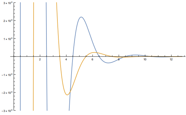
Above figures describes even(blue) and odd(yellow) equations in order. Below table shows obtained energy values in planck unit.

order	even	odd
1	0.4999999999995734	1.49999999988478779
2	2.4999999993631558	3.49999995304951438
3	4.4999998614965082	5.49999509658429805
4	6.4999895475710369	7.49979373580527079
5	8.4996333274879466	9.49569805353082541
6	10.492816893317857	11.4471134019389483
7	12.393386755815509

Therefore, there are 13 bound states: 7 even, 6 odd. As energy grows, the values get lower thatn the well-known result of half integer. To obtain real values, one can just multiply $\hbar \omega$ to each values.

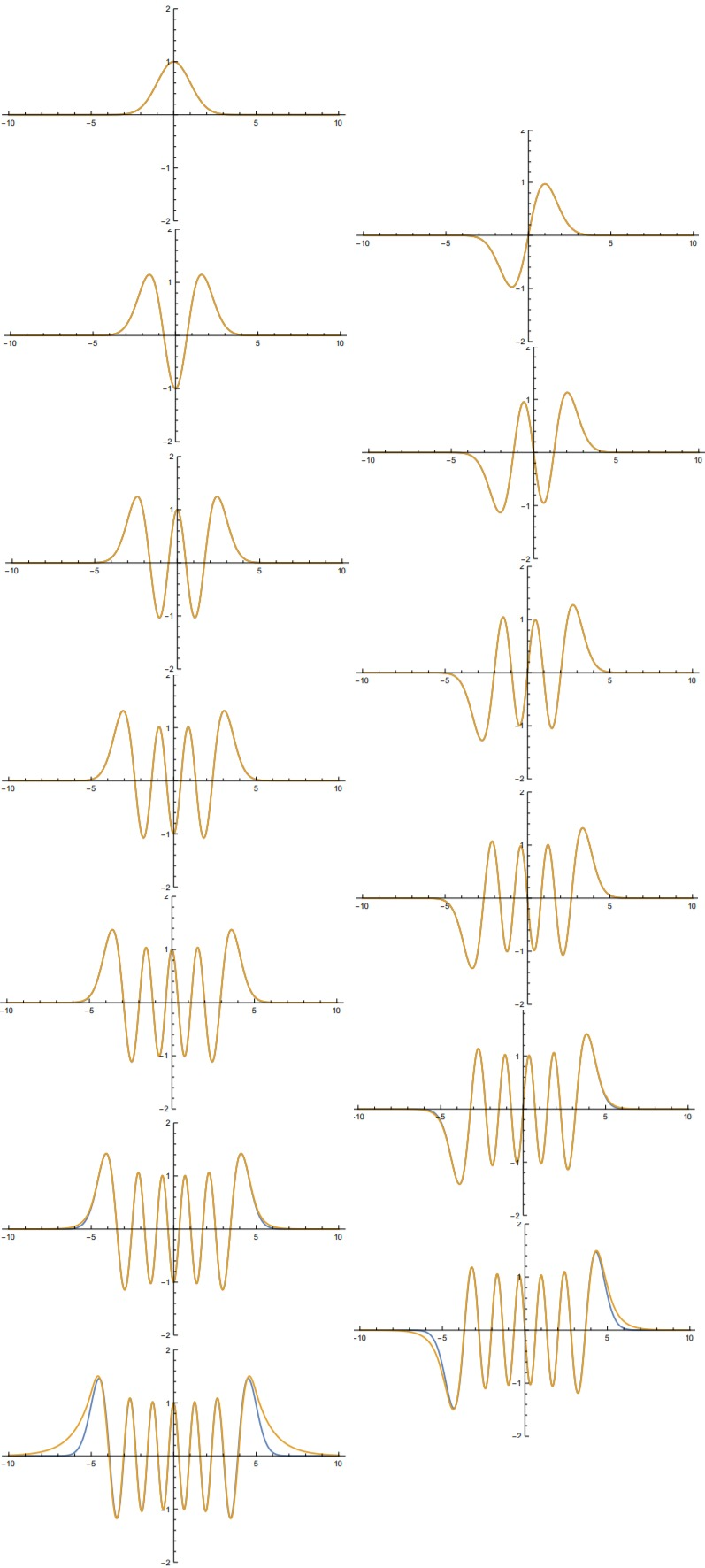
Wave functions

Here are the results of wave function. Blue line indicates the wave function for normal harmonic oscillator, and yellow lines indicate the wave functions of potential well that we were handling.

Conclusion

This result is considered reasonable. Consider the difference between infinite square well and finite square well. In this case, finite square well allows energy slightly below than infinite ones. Expecting lower energy from finite well is plausible.

On the other hand, the well’s depth almost has no effect on lower-energy states. This also sounds right, since radius of Hydrogen is $5.3\times10^{-11}$, the boundary of the well is almost 100 times larger than this. For electron in low energy state, surely this potential well must look like infinite.

Also, finite harmonic well allows broad range of region for electron especially when energy gets higher. This can be easily guessed, as energy difference gets smaller in finite well.

Reference

1. G. B. Arfken and H.-J. Weber, Mathematical methods for physicists. Elsevier Acad. Press (2011)
2. D. J. Griffiths and D. F. Schroeter, Introduction to quantum mechanics. Cambridge University Press (2019)
3. “Parabolic cylinder function” Wikipedia, (Accessed: 2019.03.2)
4. W.-P. Yuen, Exact analytic analysis of finite parabolic quantum wells with and without a static electric field Phys. Rev. B, vol. 48, no. 23 (1993)